MScene Library Documentation
Table
of Content
2.
Working with Data: Overview
2.1
Single-Data Columns and Multi-Data Columns
2.3
Importing ASCII Files into Data Tables
3.1
Cartesian and Polar 2D Graphs
3.4
Drawing Rectangles, Circles and Ellipses
4.
Drawing in 3D: Overview of the Scene
4.1
Cartesian, Polar and Cylinder 3D Graphs
4.4
Creating Polygonal Objects
4.9 Real
Time Rendering and Video Clip Recording
4.10 Printing
Images: Options for Windows 9X/ME and NT/2K
5. Using
Forms to Set Data: Overview
8 Using
Special Functions with MScene
A.6
Testing Depth and Transparency for Objects
B.1
Styles for Line Strip Objects
B.2
Styles for Polygonal Objects
B.3
Filling Modes for Polygonal Objects
B.4
Styles for Quadric Objects
C.1
Cartesian 2D Axis Orientation and Type
C.2 Polar
2D Axis Orientation and Type
C.3
Radial 2D Axis Orientation and Type
C.9 3D
Axis Orientation and Type
D.1 2D
Curves: General Properties
D.6 3D
Curves & Surfaces: General Properties
D.7
Filling Modes for Surfaces
D.8
Connecting Vertexes with 3D Curves
D.9
Coloring 3D Curves & Surfaces
D.10
Using Symbols with 3D Curves & Surfaces
D.11
Using Vectors with 3D Curves & Surfaces
E.3 Light
Properties: Ambient Component
E.4 Light
Properties: Diffuse Component
E.5 Light
Properties: Specular Component
F.1 Customizing Data Tables: General Properties
F.2
Customizing Plot Pages: General Properties
F.3 Customizing Scenes: General Properties
F.4 Customizing Scenes: OpenGL Properties
© Copyright 2005, University of California, Davis
1. Ove rview
of MScene
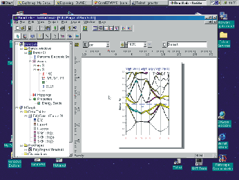
MScene is a dynamical library that performs data visualization. The data are given by sets of columns and rows. It is a plotting software that can be used to draw publication-quality 2D and 3D graphs. It is important part of the MStudio framework since all possible application libraries can be linked to MScene visualization routines.
MScene consists of five basic windows that are used to handle the data visualization process:
- Data Tables
- Plot Pages
- Scene Pages
- Form Windows
- Fits Windows
These windows can either be created using commands of Project
menu or using buttons of the MScene toolbar.
 MScene library has access to a set of
user-defined variables
seen within the scope of all MStudio windows. If data are given in terms of
(semi) analytical forms or expressions, which are used by many Data Tables, the
variables can be introduced, used and modified in one place without a need to
modify them in each particular window. Another example of the use of variables
in the graphical representation of data is to trace changes when one of the
variables is changing.
MScene library has access to a set of
user-defined variables
seen within the scope of all MStudio windows. If data are given in terms of
(semi) analytical forms or expressions, which are used by many Data Tables, the
variables can be introduced, used and modified in one place without a need to
modify them in each particular window. Another example of the use of variables
in the graphical representation of data is to trace changes when one of the
variables is changing.
MScene Library has a set of predefined special functions that can be
used to set-up data in the Data Tables. Special functions are useful for
visualizing complicated mathematical expressions, fitting the data, etc.
Special functions have to be described in a separate Dll. To create the Dll you
will need Microsoft Visual Studio 6.0 (or later ) software with Microsoft
Visual C++ installed. If you would like to use Fortran, Compaq Visual Fortran
6.0 (or later) can be used as well. A sample Dll with the description of a set
of special functions is provided with the installation of this software.
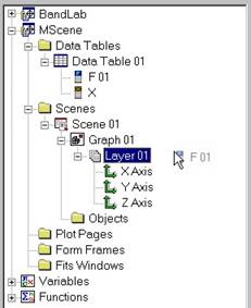
2. Working with Data: Ove rview
Data Table represents a key object of the
MScene library. Numerical data are stored in the form of tables and consist of
columns and rows.
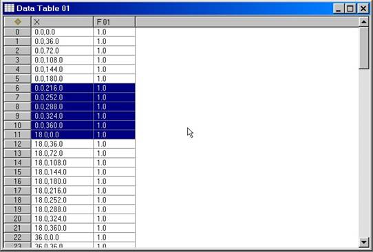
Columns in the Data Tables should be
considered as definitions of either function arguments or function values. If,
for example, a function F(x) has to be set up, a first column would represent
an argument x data, and a second column represents function value F(x) for each
argument value x. Therefore, within the framework, columns have associations,
they are associated either as arguments columns or function values columns.
Columns can also be associated as error bars if graphs should contain
information about errors. An example is the function F(x) with an uncertainty
dF(x) which can be visualized with error bars. Columns can be associated as
auxiliary. Each column has its own title. By default the first column is called
“X” and associated as the argument column. The second column is called “F01”
and associated as the function value column. The third column created would
have a name “F02”, etc. Columns are registered with the object explorer. The
column titles can be changed with the object explorer. Click on the column
icon, and then click the right-mouse button, a pop-up menu appears. Using
commands of the pop-up menu column titles and associations can be changed.
Data Tables can be set up using Form
Windows.
ASCII Files can be easily imported into
the Data Tables. Read about importing ASCII filesmscene_data_import for more detailed discussion.
2.1 Single-Data Columns and Multi-Data Columns
Each cell within the column can contain
one or a few numerical values. If column cell contain one numerical value, it
is called single-data column. If column cells contain several numerical values,
it is called a multi data column. For defining the function F(x) it is
sufficient to set up one single data column to define an argument x, and one
single-data column to define function value F(x). An advantage in using
multi-data columns is clear if one wants to consider a family of similar
functions F(x,i), i=1,N. If the latter is desired, instead of defining N single
data columns for each F(x,i), one can define a multi-data column to set up N
function values F(x,i). Within every cell commas should separate these N
values.
Multi data columns are more simple in
visualizing large sets of data, since commands to draw function F(x,i), i=1,N
are issued only once, instead of N times. Also customization of the graph can
be done once instead of N times.
Another application of multi data columns
is its use in visualizing 2D and 3D data sets. For example, to draw a surface
F(x1,x2) we consider the argument column as two-data column which contains
values x1,x2, and function value column F which is a single data column. For
the family of surfaces Fi(x1,x2), I=1,N, two-data argument column and N-data
function columns should be considered. Similar definitions are valid for
considering cross-section plots F(x1,x2,x3)=F0. A three-data column with x1,
x2, x3 values in each cell should be defined.
2.2 Handling Columns and Rows
Columns can be added to the table by
double clicking in a place separating two columns. A mouse cursor will prompt
you by changing its form from a simple arrow to an insertion form. Columns can also be added by using Add
Columns command of the Table menu.
Rows can be added to the table by double
clicking in a place separating two rows. A mouse cursor will prompt you by
changing its form from a simple arrow to an insertion form. Rows can also be
added by using Add Rows command of the Table menu.
Columns and rows can be cut, copied and
pasted using standard editor commands: pressing the right-mouse button a
corresponding pop-up menu appears.
Cells can be cut, copied and pasted in the
same way.
2.3 Importing ASCII Files into Data Tables
ASCII files can be imported to the data
tables using Import ASCII command of the Table menu. A
corresponding dialog box appears. If the ASCII file contains information about
number of columns and roots, column names and associations with a predefined
format, there is no more steps to be done, the button Import Now can be
clicked.
Predefined format for the ASCII files
reads as follows:
1.
First record sets the number of columns and rows.
2.
Second record sets number of data for each columns.
Single-data columns contain one data value per column. Multi-data columns may
contain more data values. Refer to topic Single-Data and Multi-Data Columns for more
detailed discussion. Note that the argument columns should be single-data
columns for 2D plots of functions F(x). They should be two-data columns for 3D
plots of surfaces F(x,y) and 3D curves F(x,y). For the case of surfaces, data
(x,y) should represent a 2D grid with not necessarily equidistant step. For 3D
cross-sections plots F(x,y,z)= const. the argument data (x,y,z) should be
three-data columns and represent a 3D grid with not necessarily equidistant
step.
3.
Third record contains column titles for each column. The
column titles should be separated by blanks.
4.
Fourth record contains column association information. The
following numbers give predefined column associations: 1-argument, 2-function
value, 3- error bar, 4-auxiliary.
5.
The table of data follows after first four control records
described above.
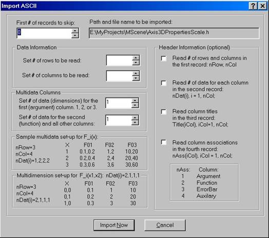
For generally organized ASCII files, the
numbers of columns and rows, as well as the numbers of data for each column
should be set manually. In this case, the first column would be assumed to be
the argument column, while second and all other columns are assumed to be the
function value columns.
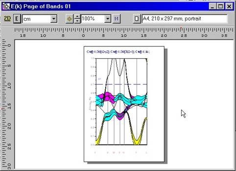
3. Plotting 2D Data: Ove rview
2D data visualization is done using Plot
Pages of the MScene library. Choosing a Plot Page command of the Project
menu creates the plot page. The window represents a graphical editor. The
following objects can be created within it:
·
Cartesian Graphs
·
Polar Graphs
·
Text Objects
·
Lines
·
Rectangles, circles and ellipses
 Choosing a
corresponding tool on the Plot Toolbar or using Select Tool command of the Plot
menu creates the objects. Choosing an arrow mode allows resize, cut, copy,
paste, delete, select, and move objects on the page. All objects are
automatically registered with the Object Explorer.
Choosing a
corresponding tool on the Plot Toolbar or using Select Tool command of the Plot
menu creates the objects. Choosing an arrow mode allows resize, cut, copy,
paste, delete, select, and move objects on the page. All objects are
automatically registered with the Object Explorer.
Data visualization is done using
the following steps:
·
Set up function F(x) using the Data Table.
·
On the Plot Page draw a Cartesian or polar graph region.
·
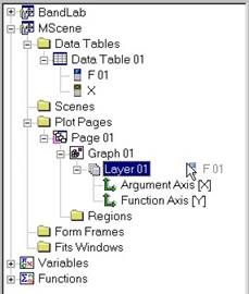
Open the data table and the plot page with the Object
Explorer, both the columns and the graph should be presented as tree items in
the object explorer. Open the graph region, it should consist of layers. Layer
1 is automatically created. If you need more layers use right-button pop-up
menu within Object Explorer when graph icon is selected.
·
Drug icon representing function value column and drop it to
the desired layer of the graph. Function F(x) should be plotted within the Plot
Page.
3.1 Cartesian and Polar 2D Graphs
 2D Graphs are the
objects of Plot Pages. Choosing a corresponding graph tool on the Plot Toolbar
or using Select Tool: Graph or Select Tool Polar Graph command of the Plot menu
creates them.
2D Graphs are the
objects of Plot Pages. Choosing a corresponding graph tool on the Plot Toolbar
or using Select Tool: Graph or Select Tool Polar Graph command of the Plot menu
creates them.
2D Graphs represent complicated objects;
they consist of bounding rectangle and layers. Adding background color and/or
frame can customize bounding rectangle. Layers are used to draw curves.
When graph is created layer 1 is created
automatically. To add more layers, find the graph object on the Object
Explorer, click right mouse button, and chose Add Layer command.
Layers consist of axes and curves. Each
layer has its own coordinate system set up by argument axis and function axis.
When layer is created the argument and function axes are created automatically.
Each layer must have one argument and one function axis. Other auxiliary axes can be added to
the layer but they do not affect the coordinate system. To add an axis, find a
particular layer in the Object Explorer, click right mouse button and chose Add
Axis command of the pop-up menu.
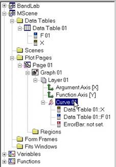
Curves are the objects that represent data
visualization. The curves are not created automatically when layer is created.
They can be added to the layer either by dragging the column icons from the
data table and dropping them to the layer icon, or by clicking right mouse
button and choosing Add Curve command of the pop-up menu. The curves are
the objects that are linked to corresponding columns of data tables. Each curve
has a link to argument column, function column, and optionally, error bar
column. To draw or redraw curves within the layer, the link between curve
object and the column objects has to be set up or modified. To set up/modify
the link, drug icons representing the columns and drop them within the curve
icons of the Object Explorer.
To customize axes and curves, select them
within the Plot Page by double clicking or use Properties command of the
pop-up menu within the Object Explorer.
The following property pages are
used for axis customization
·
Cartesian Axis Orientation and Type
·
Polar Axis Orientation and Type
·
Radial Axis Orientation and Type
·
Cartesian and Radial Axis Scale
·
Polar Axis Scale
·
Axis Ticks
·
Axis Labels
·
Axis Grid
The following property pages are
used for 2D curves customization:
·
Curves: General Properties
·
Curves Appearance
·
Curves Symbols
·
Curves Error Bars
·
Curve Limits
3.2 Adding Text
Text can be added to the Plot Pages. Chose
text tool on the Plot Toolbar or use Select Tool: Text command of the Plot
menu. Click at a place of the Plot Page where the text should appear, a text
editor will be called. Type text within the text editor using available fonts
and colors. After typing is done, click OK, and the text will appear on the
Plot page. It can be moved, resized and modified by clicking on the text object
again.
3.3 Drawing Straight Lines
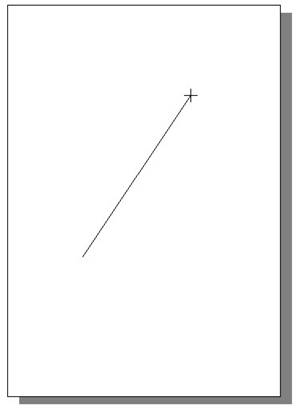 Lines can be drawn
on the Plot Pages. Chose line tool on the Plot Toolbar or use Select Tool:
Line command of the Plot menu. Arrows can be added at the beginning
or at the end of lines. Use properties dialog box for customizing the lines
appearance.
Lines can be drawn
on the Plot Pages. Chose line tool on the Plot Toolbar or use Select Tool:
Line command of the Plot menu. Arrows can be added at the beginning
or at the end of lines. Use properties dialog box for customizing the lines
appearance.
Combine line drawing with the Shift key to
obtain horizontal or vertical lines. The line objects can be moved, resized and
modified by clicking (double clicking) on them.
3.4 Drawing Rectangles, Circles and Ellipses
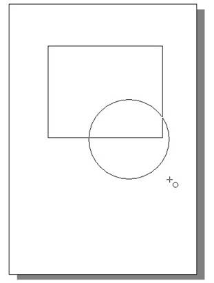 Rectangles,
circles and ellipses can be drawn on the Plot Pages. Chose either Rectangle or
Circle tool on the Plot Toolbar or use Select Tool: Rectangle, Circle command
of the Plot menu. Use properties dialog box for customizing appearance
of these objects. Combine drawing with the Shift key to obtain proper figures.
These objects can be moved, resized and modified by clicking (double clicking)
on them.
Rectangles,
circles and ellipses can be drawn on the Plot Pages. Chose either Rectangle or
Circle tool on the Plot Toolbar or use Select Tool: Rectangle, Circle command
of the Plot menu. Use properties dialog box for customizing appearance
of these objects. Combine drawing with the Shift key to obtain proper figures.
These objects can be moved, resized and modified by clicking (double clicking)
on them.
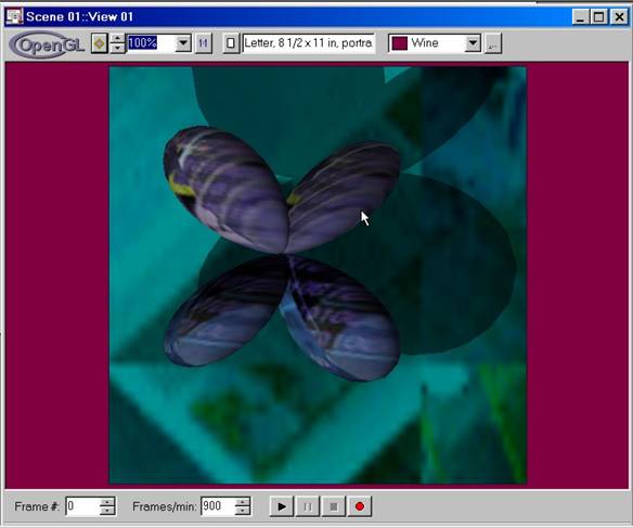
4. Drawing in 3D: Ove rview
of the Scene
3D data visualization is done using Scene
Pages of the MScene library. Choosing a
Scene Page command of the Project menu creates the scene page. The window
represents a 3D graphical editor.
The key object on the Scene Page is the
Scene itself. We understand by the scene a cube with Cartesian coordinate
system spanning from left to right for x-axis, from bottom to top for y axis
and from far to near for z-axis (perpendicular to the screen and pointing to
the eyes). The scale for all axes is assumed to be the same varying from –1 to
1. The point (0,0,0) is thus the center of the screen. By introducing the
coordinate system we can place any object within this 3D space. We associate a
bounding cube with every object. We consider the following operations for this
cube: scaling along x,y,z axes, shift away from the central point and rotation
around x,y,z axis. If no scaling, no shift, no rotation exists, the object cube
on the scene is assumed to span from –0.5 to +0.5 along every direction and
occupies precisely 1/8 part of the scene volume.
The following objects can be
created within the Scene:
·
Cartesian Graphs
·
Polar Graphs
·
Cylinder Graphs
·
3D Text Objects
·
Line Srip Objects: lines, cubes, etc.
·
Polygonal Objects: cubes, balls, polygons, etc.
·
Quadric Objects from the library
·
Scene Objects: how to convert the whole scene into single
object
·
Light Objects: how to lighten the scene
·
Wall Objects: how to create shadows
Choosing corresponding tools on the Plot
Toolbar or using Select Tool command of the Scene menu creates the objects.
Choosing an arrow mode allows resize, cut, copy, paste, delete, select, and
move objects on the page. All objects are automatically registered with the
Object Explorer.
The objects can be moved within the scene,
colored, lightened and made semitransparent. The objects surfaces can be
fogged, and textured with images. You will need standard Windows bitmap file
that contains desired image to put it onto the object surface. If you create
scene walls the objects can show up their shadows from all light sources
existing on the scene.
The objects on the scene appear with some
default behavior. Most of these properties can be by customizing the Scene
property pages. To call scene property pages, either click right arrow button
when no objects are selected or use command Properties within the Scene
menu. The Scene can be customized using the following property pages
·
Scene Projection
·
Objects Static Positions
·
Objects Time-Dependent Positions
·
Appearance of Objects
·
Depth Function for Objects
·
Object Shadows
·
Fog Effect
The scenes can have multiple views. Choose
Add View command from the Scene menu to add another view to your scene.
When all views of the scene are closed the scene does not disappear
automatically. You can delete the scene from the Object Explorer by choosing Delete
command from the right-mouse pop-up menu when selecting the scene icon.
Multiple views are useful to view the scene from different angles. You can
spontaneously view the scene from the front and from the left, for example. You
can move the object at one view and see how they are moving at another view
under different view angle.
Another option of the scene is real time
rendering.
Objects positions and colors can be made time dependent. In other words if
object position is described by the vector R=(Rx,Ry,Rz), the vector can be set
as a function of time t: R(t). When player is running, time variable t is
passed to every object to determine its real-time coordinate, scaling, rotation
and color. You can record the scene into video clip and show it with your
presentations.
Printing options depend on the operating system. For
Windows 95/98/ME the only option is to capture the scene image into bitmap file
and print it with Windows MSPAINT program. For Windows NT/2K, printing can be
done directly via the use of enhanced metafile spooling.
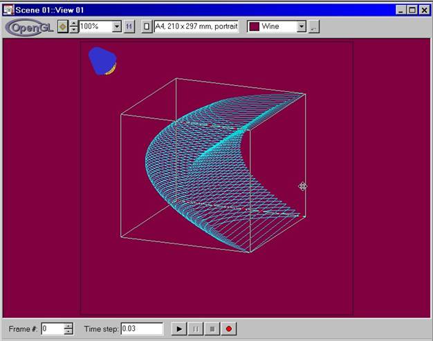
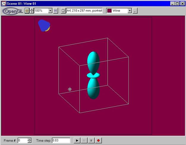
4.1 Cartesian, Polar and Cylinder 3D Graphs
3D Graphs are the objects of the Scene
Pages. They are created by choosing a corresponding graph tool on the Plot
Toolbar or using Select Tool: Graph/Polar Graph/Cylinder Graph command
of the Scene menu.
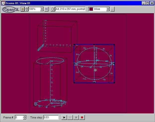
3D Graphs represent complicated objects,
they consist of bounding cube and layers. Layers consists of axes and surfaces.
Bounding cube can be customized by showing its frame and its planes. The layers
set up custom coordinate systems within 3D graph space. The coordinate systems
in use are either Cartesian (xyz), polar (rqf) or cylinder (rfz) ones. The
layers are used to plot 3D curves, surfaces and cross-sections. They may
contain several surfaces as long as the surfaces refer to the same coordinate
system. Multilayering is useful if one has several surfaces which should be
shown on top of each other within the same graph but the surfaces are defined
with different coordinate systems.
When graph is created, the first layer is
created automatically. For Cartesian graphs, the first layer created is
Cartesian, for polar graphs the first layer created is polar, for cylinder
graphs, the first layer created is cylinder. To add more layers, find the graph
object on the Object Explorer, click right mouse button, and choose Add
Layer command.
Layers consist of axes and curves. Every
layer needs three axes that are called principal axes. There can be also
auxiliary axes that play no role in defining the coordinate system within the
layer. Cartesian layer is set up by three axes, left-right (x), bottom-top (y),
and far-near(z). Polar layer is set up by radial axis r and two angular axes, q
axis
that spans from 0 to 180 degrees and f axis that spans
from 0 to 360 degrees. By default q axis is vertical
and f axis is horizontal. For cylinder layers, we have angular f
axis
that is horizontally oriented, radial r axis within the horizontal plane and
vertical z axis.
When layer is created three principal axes
are created automatically. Auxiliary axes can be added to the layer but
they do not affect the coordinate system. To add an axis, find a particular
layer in the Object Explorer, click right mouse button and chose Add Axis command
of the pop-up menu.
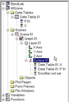
3D Curves and Surfaces are another kind of
the graph objects. The surfaces are not created automatically when layer is
created. They can be added to the layer either by dragging the column icons
from the data table and dropping them to the layer icon, or by clicking right
mouse button and choosing Add Surface command of the pop-up menu. The
surfaces are the objects that are linked to corresponding columns of data
tables. Each surface has a link to argument column, function column, and
optionally, error bar column. Error bar column can be used to color surfaces
differently according to auxiliary function associated with the surface or to
put symbols of different size (again according to auxiliary function associated
with the surface on top of the original data points.
 3D Data sets can
be visualized as 3D curves: F(x1,x2), surfaces: F(x1,x2) and cross-sections:
F(x1,x2,x3)=const. For surfaces and cross-sections the argument data sets
(x1,x2) or (x1,x2,x3) should represent proper 2D or 3D grids with not
necessarily equidistant steps. We may also consider whole families of
surfaces Fj(x1,x2) or
Fj(x1,x2,x3)=const., j=1,N. The advantage of dealing with such data set is that
the customization procedure should be done only once for the whole family of
surfaces. The function value columns should contain N data values in this case.
3D Data sets can
be visualized as 3D curves: F(x1,x2), surfaces: F(x1,x2) and cross-sections:
F(x1,x2,x3)=const. For surfaces and cross-sections the argument data sets
(x1,x2) or (x1,x2,x3) should represent proper 2D or 3D grids with not
necessarily equidistant steps. We may also consider whole families of
surfaces Fj(x1,x2) or
Fj(x1,x2,x3)=const., j=1,N. The advantage of dealing with such data set is that
the customization procedure should be done only once for the whole family of
surfaces. The function value columns should contain N data values in this case.
Visualization process is done using
the following steps:
·
Set up function F(x1,x2) or F(x1,x2,x3) using the Data
Table.
Note that argument column should contain two-data or three-data set here
describing the values x1,x2 or x1,x2,x3.
·
On the Scene Page draw a Cartesian, polar or cylinder graph
object.
·
Open the data table and the scene page with the Object
Explorer, both the columns and the graph should be presented as tree items in
the Object Explorer. Open the graph region, it should consist of layers. Layer
1 is automatically created. If you need more layers use right-button pop-up
menu within Object Explorer when graph icon is selected.
Drug icon representing function
value column and drop it to the desired layer of the graph. A dialog box should
appear asking whether a 3D curve, surface or cross-section should be drawn. For
the cross-section, additional contour value F0=F(x1,x2,x3) should be entered.
The 3D Graph should appear within the Scene Page shortly.
 The surfaces can
be colored according to the auxiliary functions associated with them. The
possibility also exist to draw symbols and/or vectors at each surface point
according to the auxiliary functions. To take this effect, first add the
auxiliary function column A(x1,x2) or A(x1,x2,x3) (or their multidata analogs)
to the data table. Associate those columns with the errorbar data and connect
them to the surface. After this, the surface can be colored or symbols of
variable size can be placed at each surface vertex. To draw vectors one
generally has to set up the vector field Ax1(x1,x2,x3), Ax2(x1,x2,x3),
Ax3(x1,x2,x3) and set it as the errorbar column. This assumes that
the errorbar column is already a multidata column. The vectors can now be drawn
and oriented according to the vector field attached to the surface. This
procedure is also generalized to the multidata cases for surface families Fj(x1,x2,x3),
j=1,N, when the vector fields are set up by Ax1,j(x1,x2,x3), Ax2,j(x1,x2,x3),
Ax3,j(x1,x2,x3), j=1,N
The surfaces can
be colored according to the auxiliary functions associated with them. The
possibility also exist to draw symbols and/or vectors at each surface point
according to the auxiliary functions. To take this effect, first add the
auxiliary function column A(x1,x2) or A(x1,x2,x3) (or their multidata analogs)
to the data table. Associate those columns with the errorbar data and connect
them to the surface. After this, the surface can be colored or symbols of
variable size can be placed at each surface vertex. To draw vectors one
generally has to set up the vector field Ax1(x1,x2,x3), Ax2(x1,x2,x3),
Ax3(x1,x2,x3) and set it as the errorbar column. This assumes that
the errorbar column is already a multidata column. The vectors can now be drawn
and oriented according to the vector field attached to the surface. This
procedure is also generalized to the multidata cases for surface families Fj(x1,x2,x3),
j=1,N, when the vector fields are set up by Ax1,j(x1,x2,x3), Ax2,j(x1,x2,x3),
Ax3,j(x1,x2,x3), j=1,N
If vector field is set, the symbols
can be drawn and scaled proportionally to the absolute value of the field. The
same can be done for coloring the surface. If, on the other hand, only scalar
field is set as the auxiliary function, the vectors can be drawn by either
constant orientation, or perpendicular to the surface.
To customize axes and surfaces,
select the corresponding icons within the Object Explorer by double clicking or
use Properties command of the pop-up menu.
The following property pages are
used for axis customization:
·
Axis Orientation and Type
·
Axis Scale
·
Axis Ticks
·
Axis Labels
Since every axis is considered as
the Scene object, the following object property pages are also applied to axis
customization:
·
Appearance of Objects
·
Depth Function for Objects
·
Object Shadows
·
Fog Effect
The following property pages are
used for surfaces customization:
·
Surfaces General Properties
·
Filling Modes for Surfaces
·
Using Symbols with Surfaces
·
Using Vectors with Surfaces
·
Coloring Surfaces
·
Connecting Vertexes with 3D Curves
Since every surface is considered
as the Scene object, the following object property pages are also applied to
surfaces customization:
·
Appearance of Objects
·
Texture of Objects
·
Depth Function for Objects
·
Object Shadows
·
Fog Effect
Graph objects themselves can be
customized in a similar way. The following property pages are applied for them:
·
Graph Styles
·
Objects Static Positons
·
Objects Time-Dependent Positions
·
Appearance of Objects
·
Texture of Objects
·
Depth Function for Objects
·
Object Shadows
·
Fog Effect
4.2 Adding 3D Text
3D text can be drawn within the Scene
Page. Chose text tool on the Plot Toolbar or use Select Tool: Text command
of the Scene menu. Click at a place on the Scene Page where the text
should appear, a text editor will be called. Type text within the text editor
using available fonts and colors. After typing is done, click OK, and the text
will appear on the Scene page. It can be moved, resized and modified by
clicking on the text object again.
Since3D text is considered as one
of the scene objects, the following property pages can be applied to customize
text appearance:
·
Text Style
·
Objects Static Positons
·
Objects Time-Dependent Positions
·
Appearance of Objects
·
Texture of Objects
·
Depth Function for Objects
·
Object Shadows
·
Fog Effect
4.3 Creating Line Strips
Line strips are the objects that are
constructed from a set of connected lines. A set of preconstructed line strips
such as cube or tetrahedron exists with the installation of the program.
Navigate the folder …/Scene Data/Line Strips to see the files with the
extension *.lin.
There are several ways to construct your
own line strip objects: use ASCII editor to describe coordinates of the
vertexes, use line strip editor, which is simply given by the tree control, or
convert any 3D curve drawn within the 3D graph object into the line strip
object.
When you select a line strip tool on the
Plot Toolbar or use Select Tool: Line Strip command of the Scene
menu, the default line strip object (a cube) is created. Double click on the
object or use right-mouse pop-up menu button to call Properties Dialog box. The
line strip style property page
allows you to navigate through the database of the line strip objects. It also
includes a simple tree control that allows you to create/modify/remove these
objects.
Since the line strip objects are stored in
the …/Scene Data/Line Strips folder you can modify them directly with any ASCII
editor. Another option is to convert a 3D curve into the line strip object:
Find the 3D curve icon within the Object Explorer, and use right-mouse
button pop-up menu to call Export As Object command. You will need to
entitle your line strip object and choose the folder to store it. The best way
is to store it within the same database in the ../Scene Data/Line Strips
folder.
The following property pages can be
applied to customize line strips appearance:
·
Line Strip Style
·
Objects Static Positons
·
Objects Time-Dependent Positions
·
Appearance of Objects
·
Texture of Objects
·
Depth Function for Objects
·
Object Shadows
·
Fog Effect
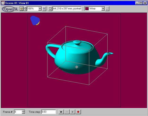
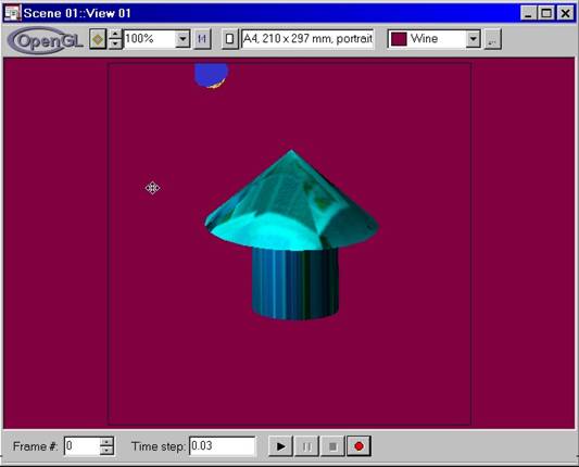
4.4 Creating Polygonal Objects
Polygonal objects are the objects that are
constructed from a set of polygons. A set of preconstructed polygons such as
cube or tetrahedron exists with the installation of the program. Navigate the
folder …/Scene Data/Polygons to see the files with the extension *.pol.
There are several ways to construct your
own polygonal objects: use ASCII editor to describe coordinates of the
vertexes, use polygons editor, which is simply given by the tree control, or
convert any surface drawn within the 3D graph object into the polygonal object.
When you select a polygon tool on the Plot
Toolbar or use Select Tool: Polygon command of the Scene menu,
the default polygonal object (a cube) is created. Double click on the object or
use right-mouse pop-up menu button to call Properties Dialog box. The polygon
style property page
allows you to navigate through the database of the polygonal objects. It also
includes a simple tree control that allows you to create/modify/remove these
objects.
Since the polygonal objects are stored in
the …/Scene Data/Polygons folder you may modify them directly with any ASCII
editor. Another option is to convert a surface into the polygon object: Find
the surface icon within the Object Explorer, and use right-mouse pop-up
menu to call Export As Object command. You will need to entitle your
polygonal object and choose the folder to store it. The best way is to store it
within the same database in the …/Scene Data/Polygons folder.
The following property pages can be
applied to customize polygons appearance:
·
Polygons Style
·
Polygons Filling Modes
·
Objects Static Positons
·
Objects Time-Dependent Positions
·
Appearance of Objects
·
Texture of Objects
·
Depth Function for Objects
·
Object Shadows
·
Fog Effect
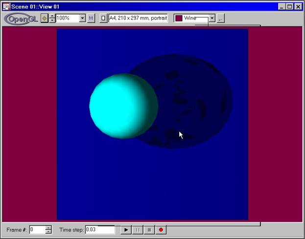
4.5 Creating Quadric Objects
Quadric objects such as cylinders and
balls are drawn using OpenGL utility library. There is no way to modify these
objects directly but you can resize them and customize their appearance.
When you select a Quadric tool on
the Plot Toolbar or use Select Tool: Quadric command of the Scene
menu, the default quadric object (a ball) is created. Double click on the
object or use right-mouse pop-up menu to call Properties Dialog box. The
quadric style property page
allows you to choose various quadric objects from the library as well as
customize their size and appearance.
The following property pages can be
applied to customize quadric appearance:
·
Quadric Style
·
Objects Static Positons
·
Objects Time-Dependent Positions
·
Appearance of Objects
·
Texture of Objects
·
Depth Function for Objects
·
Object Shadows
·
Fog Effect
4.6 Creating Scene Objects
When scene composition is done one can
store the scene as a single object. This allows you to construct complicated
objects from the primitive ones for future reuse. To convert the whole scene
into single object use Save As Object command within the Scene menu.
You will need to entitle your scene object and it will be stored in the Scene
Database located at .../Scene Data/Scenes.
To draw a scene object within the current
scene, select Scene tool from the Plot Toolbar or use Select
Tool:Scene command of the Scene menu. The default scene object (a
cube) is created. Double click on this object or use right-mouse pop-up menu to
call for Properties Dialog box. The scene style property page allows you
to choose various scene objects from the scene objects database as well as to customize
their size and appearance.
Note that light objects and walls are not
participated in this conversion.
The following property pages can be
applied to customize scene objects:
·
Scene Style
·
Objects Static Positons
·
Objects Time-Dependent Positions
·
Appearance of Objects
·
Texture of Objects
·
Depth Function for Objects
·
Object Shadows
·
Fog Effect
4.7 Adding Light to Scene
Lighting is one of the most important
elements in adding realism to your scenes. Use Light tool from the Plot
Toolbar or use Select Tool: Light from the Scene menu to add
light sources to your scene. You can add total up to 8 light sources that is
the current limitation of OpenGL windows implementation.
Lighting of the objects depends on the
normals to the surfaces. Therefore some care should be taken when you define
surface normals to your objects. It may happens that the lighting effect works
completely opposite to what you expect, you are trying to lighten one side of
the surface but see lightened completely opposite part. That precisely means
that normals are chosen in the opposite way. Every object has a possibility to
choose normals in either one or another way. That is especially important for
surfaces and cross-sections where a priori it is not clear which part of the surface is
front and which one is back.
Lighting icons appear on the scene as
small bulbs. You can move them within the scene, and by default the light spot
is pointing at the scene center, point (0,0,0) at the scene coordinates. You
can remove the light icons by toggling Light Bulbs command within the Scene
menu.
The following property pages can be
applied to customize the light sources:
·
Light Spot
·
Light Model
·
Ambient Component
·
Diffuse Component
·
Specular Component
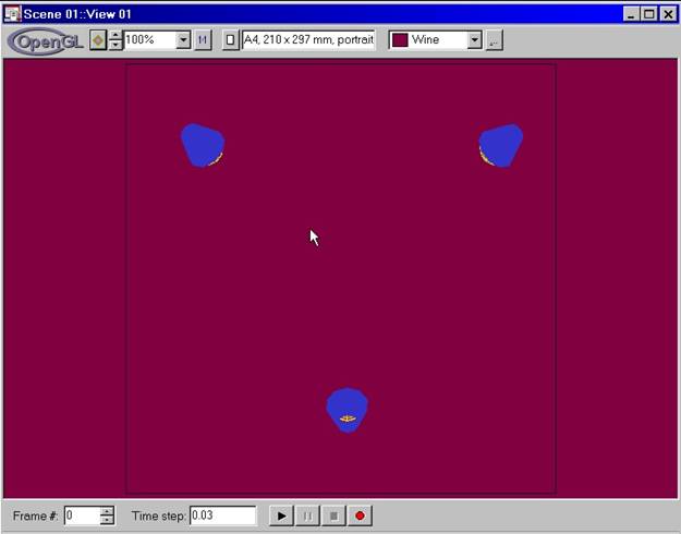
4.8 Scene Walls and Shadows
Objects shadows can be made easy. To
create a shadow we need an object, a light source and a wall. The walls are
scene objects, which are just planes. They are considered as special type of
polygonal objects and can be customized in a way similar to all polygonal
objects. One difference is that the wall object defines the plane in 3D space
in which shadows can appear. Shadows are considered to be objects flattened on
the wall plane. They can have certain color and transparency but they are
bounded to the position of the object, position of the light source and
position of the wall plane. Note that if you create several walls and use
several light sources, every object will create its shadow on every wall from
every light source. You can customize shadows and make them semitransparent
which looks usually very cool.
The wall objects can be customized
using the following property pages:
·
Polygons Style
·
Objects Static Positons
·
Objects Time-Dependent Positions
·
Appearance of Objects
·
Texture of Objects
·
Depth Function for Objects
·
Fog Effect
4.9 Real Time Rendering and Video Clip
Recording
Every scene window has a player toolbar at
its bottom. When you press onto PLAY button you see the scene is rotating and
changing its size. This effect is implemented by considering positions of every
object including the scene itself to be time-dependent. When you see your scene
statically, it is shown at the time moment t=0. When you press PLAY button, a
separate thread is started which consists of the looping cycle. The looping is
performed with increasing time variable t passed to every object which
determines the object coordinates at time moment t. Every frame shown when
player is running represents a time slice with the objects positions determined
at the given time moment t. You can vary time step dt so that the next frame
will be shown at the time moment t+dt. Increasing dt will accelerate the
objects movement at decreasing dt will slow down the movements.
Every object position is described by the
scaling factors along x,y,z directions, the shift vector from the origin and by
the rotations along x,y,z axis. We distinguish static part in this description
and the dynamic part. So that the final scaling of the object along, say, x direction,
Sx(t) is represented as a product S0x * STx where S0x is the static scaling and
STx is the dynamic scaling. For example, if S0x=1, and STx=cos(t)*cos(t), the
object will be scaling from 1 to 0 and back to 1 along x-direction. For shifts
and rotations we use sums of the static and dynamic components. For example to
rotate the object around z-axis with time, we set R0z=0 and RTz=10*t, so that
the total rotational angle Rz(t)=R0z + RTz = 10 *t which is zero at t=0 and is
increasing function of time.
Static components of the object
position are set by the Positon Property Page.
Time-dependent components of the object position are set by the Time Property PageHIDD_GLYPH_PROPERTIES_TIME.
Note that we also consider static and
dynamic components for the object colors. This works very well for the alpha
(transparency) components so that you can reach really cool effect of the
object disappearance by setting the static alpha component equal to 1 and
time-dependent component to cos(t)*cos(t).
Static components of the object
color are set by the Appearance Property Page.
Time-dependent components of the object color are set by the Time Property Page.
Scene itself can also have its position in
time, so that scaling shift and rotational elements are defined not only for
every object but also for the whole scene. That means that if object position
is determined with respect to the scene (another option is to set it with respect
to the screen) the final object position at time moment t involves as the
positions of the object with respect to the scene coordinates and the position
of the scene with respect to the screen coordinate. So that if the object is
oscillating within the scene and the scene is rotating around some axis you
should see the rotating scene with oscillating object inside. If object
position is determined with respect to the screen, the scene will be rotating
but the object inside it will be oscillating without following the scene
movements. You can write your own scenarios for your object movements and store
them within …/Scene Data/Time Function database. See the description of Time
Property Pages
to find out more.
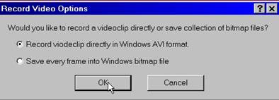
You can record video for the scene using
RECORD button of the player toolbar. The video clip can be recorded either as a
set of frames or as Windows AVI file. If you choose to record your video in a
set of frame, this creates a set of Windows bitmap files entitled according to
the frame number. You can further compose a video from these frames using
another Windows software. If you choose to create a Windows AVI file, your
video clip will be recorded with each frame 2/3 of seconds apart and you can
play it directly using Windows media player. Watch out for the size of the file
since usually uncompressed video clips take a lot of disc storage. You can
significantly reduce the disc storage of your video clips by converting your
AVI files to MPEG format.
4.10 Printing Images: Options for Windows 9X/ME
and NT/2K
Printing your images is done by the
standard facilities of the Windows operating system. For OpenGL based
applications direct printing to the printer devices is implemented via the
enhanced metafile spooling. The latter option is currently implemented by
Windows NT/2K operating systems only. It is advantageous due to the fact the
enhanced metafile commands are the vector commands that represent recorded
OpenGL command sequence. However it may take a significant amount of disc
storage and time to print complicated 3D images directly to the printer.
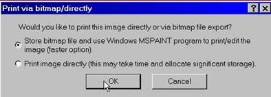
The easiest and fastest option in printing
your images is via native Windows bitmap files support. This option works well
on both Windows 9X/ME and NT/2K families of operating systems. If you choose
this option, your image will be stored as a bitmap in a raster format and the
standard Windows MSPAINT program will be called. You can reorient, scale, and
edit your bitmapped image using that program as well as use all printing
options available.
5. Using Forms to Set Data: Ove rview
Forms are MScene windows used to set-up
and manipulate data within the Data Tables. These can be used to set up column
values, to add and subtract columns, multiply columns by numbers and perform other
operations.
Forms are separated into three parts:
Upper control part is used to set up target columns and select rows and data
participating in transformation. Middle part is an editor that is used for
entering expressions to be used in columns transformation. The lower control
part is used to set up 1D, 2D or 3D regular grids for the argument columns. If
grid control is used, the middle editor is not accessible.
To understand how forms are working,
consider several examples. Suppose we have a data table entitled Data Table 01
with two columns, the argument column X and the function column F01. We would
like to set up a function F(x)=cos(x) at a set of values x varying from 0 to 1.
We first need to set up argument column x covering the interval from 0 to 1
with a step 0.01. We should have 101 rows in the data table. We select the
command DO FROM IROW TO IROW and set starting row to 0 and ending row to 100.
Then, we select a target column to be Data01::X. Then we type in the edit
field: irow/100 and press APPLY button. The table should contain column X
filled with the data from 0 to 1 with the step 0.01. We now ready to set up a
function column. We select a target column to be Data Table 01::F01. Then we
type in the edit field: cos(col(Data Table 01::x)) and press APPLY button. The
function column in the Data table should be filled with the data representing
cos(x) values. To slightly simplify the syntax we can select the default data
table in the upper control part to be Data Table 01. Then we just type in the
edit field: cos(col(x)) and the program will look at all columns in the Data
Table 01 by default to find the one entitled as “x”.
Several features are seen from considering
this example. First, variables can be used in the edit field (middle part of
the Forms Window). There are several reserved variables such as iRow and iDat
that selects which rows and data should be used. You can also use any other
variables defined for the project. (See topic Using Variables) For example variable PI=3.1415
always exists. (Navigate Variables folder within the Object Explorer to see all
the variables). We could type in principle iRow/100*pi to set up argument
column. The second feature is the use of vector-like command in the formulae that
deal with the columns. Whenever you type col(Data Table Name::Column Name),
values from the corresponding column will be selected and substituted to the
formula. You can omit the title of the data table in the column definition if
you select a default data table from the list box within the upper control
field. That explains the syntax cos(col(x)). More complicated expressions
involving brackets, etc are welcome. We could type cos(pi*col(x))
+sin(iRow/10*pi) as another example.
A set of predefined special functions can
be used in the expressions programmed within the Form Windows. (See topic Using Special Functions to see how to
set up special functions). Suppose we programmed a Bessel function which is
called using the syntax sphbes(l,x) where l is an integer value and x is a real
argument value. If we would like to set up a function column F01 to be equal to
the Bessel function for l=0, we just type in the edit field: sphbes(0,col(x))
and press APPLY button. The software will automatically call your special
function, evaluates it and substitutes the function column by the values of the
Bessel function.
Next topic to discuss is the use of the
grid control to set up argument data. For 1D,2D,3D grid the argument columns
should contain one-data, two-data and three data values. The grid control is
available for argument columns only. It is not accessible for the functions and
error bar columns. Select again X column as the target column and instead of
typing iRow/100 within the edit field, check 1D grid within the grid control.
Set up # of points to be 100, minimum value to be 0 and the maximum value to be
1. Press APPLY button. You will see that the argument column is filled with the
values of x varying from 0 to 1 with the step 0.01. 2D and 3D grid are created
similarly.
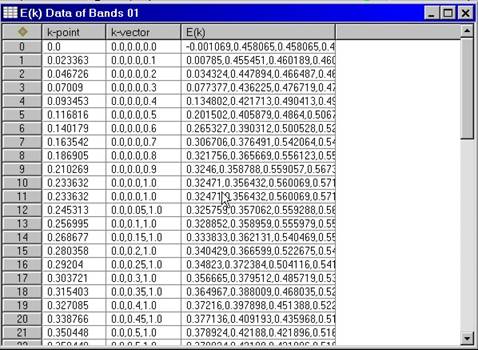
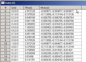
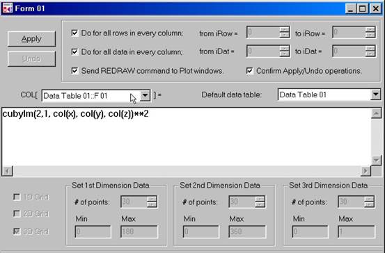
Let’s finally consider an example how we
can set up the function called cubic harmonic Y_li(Theta, Phi) related to
linear combinations o spherical harmonics which represent the solutions of the
angular part of the
Our first step is to set up an angular
grid. We create an argument column within the data table and call it TF. Then
we create a 2D grid for the target column TF varying first argument from 0 to
180 (for theta angle) and the second one from 0 to 360 (for the phi angle) with
the number of points, say, equal to 50,50.
Our second step is to set up three
auxiliary columns which would represent the vector components x,y,z. We create
three columns and call them X,Y,Z. For the target column X we use the following
formula (default data table is chosen to be data table 01):
sin(arg1(TF)/180*pi)*sin(arg2(TF)/180*pi). The syntax arg1(x) works similarly
to the syntax col(…). It takes the first argument within the specified column
(TF in this case) which represents our theta values. Therefore the whole
expression reads as sin(theta)*sin(phi) which gives the x-component for the
unit vector given by theta,phi angles. In the same way column Y is set up by
the formula sin(arg1(TF)/180*pi)*cos(arg2(TF)/180*pi) which is equivalent to
sin(theta)*cos(phi) and column Z is given by cos(arg1(TF)/180*pi) equivalent to
cos(theta).
Our last step is to evaluate the cubic
harmonic function (its square) which is given by the special function with the
notation cubylm(l,I,x,y,z). We choose a target column to be Data Table 01::F01
and type within edit field: cubylm(2,4,col(x),col(y),col(z))**2. After pressing
APPLY button the column should be filled with the values of the square of the
cubic harmonic for l=2, I=4 (proportional to x**2-y**2).
We are now ready to draw a surface
representing by the function column F01 and the argument column TF using 3D
polar coordinate system. See discussion on Cartesian and Polar 2D/3D Graphs
6. Fitting the Data: Ove rview
Data fitting is an important step in the
data analysis and visualization. Special window called Fits Window is designed
to deal with the data fits for MScene library. To call Fits Window use Fits
Window command of the Project menu or a corresponding button of the
MScene Toolbar.
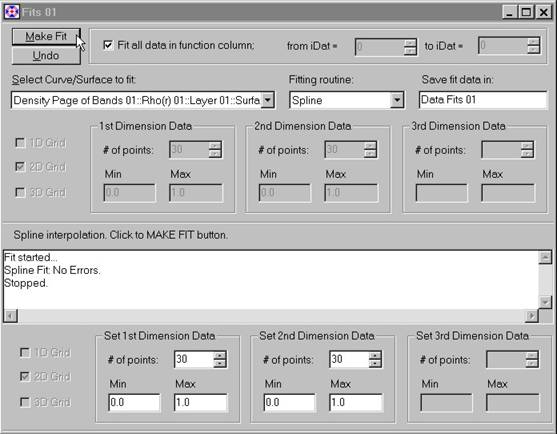
Fits window operates with 2D curves and 3D
surfaces. These are the objects consisting of argument, function values and
possibly error bars. They are linked to corresponding columns of the data
tables. The framework maintains a whole list of curves/surfaces created within
the project. Since each curve/surface has its own name, they can be easily
found. The whole curve/surface name consists of the page title, the graph
title, the layer title and the curve/surface name itself.
To make a fit from one argument grid
points to a more denser grid a spline fitting method can be used. First, select
a curve/surface that will be fitted. Use drop-down list. An original argument
grid will be shown at the upper window panel. Select new grid data at the lower
part of the fits window. Select desired interval and the numbers of grid points
Select destination table title where fits data will be stored. Press Make
Fit button. Messages from the fitting routine will appear within the fits
window area showing the fitting process. Upon successful completion the fits
data table will contain new curve/surface data. You will be asked if you would
like to link new data to the curve/surface object. If you choose YES, a
curve/surface object will be updated immediately with the fitted data. You may
undo this operation by pressing UNDO button. The curve/surface object will be
linked back to the original data columns.
7 Using Variables with MScene
A set of user-defined variables can be
specified within the project. They are extremely useful in the Form Windows. User defined
variables are the feature which allows to program expressions using mathematical
notations like cos(pi*iRow/10) with pi being the user defined variable.
Variables are useful when used by more than one form. Then, there is no need to
make changes in every form; only the variable definition has to be changed.
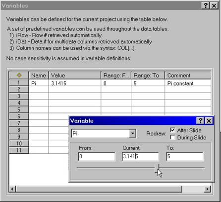
To define a variable call Variables
dialog box of the Project menu or use Variables item within the
Object Explorer. Variable has its name, value, and variation range. Comments
for the variables can be added.
If a particular expression in the Form
Window contains the variable, the variable value defined in the above way will
be used for setting up the data column(s). When variable value is being
changing, a framework will automatically reset those columns that are obtained
with the use of this variable. This way provides an interactive watch for the
plots when one of its parameter is changing.
Suppose a particular form window contains an
expression involving variable pi. This can, for example, be cos(pi*iRow/10).
The form window sets a column in a particular data table. This column can be
linked to the graph region of a particular plot page and visualizes the
function. The question now is what happens if one changes the variable
definition? Changing the variable definition will send a message to the form window
and the window will reset the variable value. Once the value is reset, the
message will be sent to the data table, and the column being connected with the
form window will update its data. Once the data in the column are updated, the
plot page window will receive an update message to redraw the plot visualizing
this column. It is therefore seen that any interactive change in the variable
value automatically redraws the graphs linked with this variable.
The only work to do here is to call a Variable
dialog box. It can be called by double clicking the variable item within the
Object Explorer. Set up range of the variable changes, and slide the vertical
bar of this dialog box. Watch for the graph that involves this variable, there
will be interactive redrawing while sliding the bar. Note that this option
works only with 2D graphics.
8 Using Special Functions with MScene
A set of user defined special functions
can be used in the expressions programmed within the project. They can be
useful for example when working with Form Windowsmscene_form_overview.
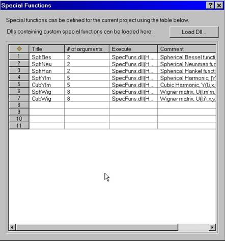
The set of special functions has to be
defined in the dynamical library SpecFuns.Dll. To create your own special
functions library you will need Microsoft Visual C++ and/or Compaq Visual
Fortran. A sample provided for creating SpecFuns.Dll is provided with the
installation of the software which is located at the folder ../Scene
Data/SpecFuns.
You can choose either language, C++ or
Fortran to program functions that you want to visualize. In fact, the sample
source code for the SpecFuns.Dll consists of mixed C++/Fortran examples. You
can link both C++/Fortran codes together and call Fortran subroutines from the
C++ and vice versa. Following this example you can create your own special
functions databases easy and quickly.
A.1 Appearance of Objects
Objects on the scene appear in
color and their surfaces reflect light. The surfaces have front and back sides,
therefore they can be colored differently and reflect the light differently.
Given set of properties is set up by the Appearance property page. Since
we do not distinguish between objects and object shadows, similar property page
exists to customize shadow appearance. If the property page is
opened for the whole scene, it will reflect the default settings that are
accumulated by the objects during creation. Properties of the object surface
are called properties of the material. If material properties are given by
default, the object accumulates the settings given by the scene. If object
material customization is enabled, mode and face parameters of the material can
be changed. If material properties are disabled, object does not appear in
color. Lighting of the object surface can be switched on/off. If lighting of
the object is off, it appears of constant color.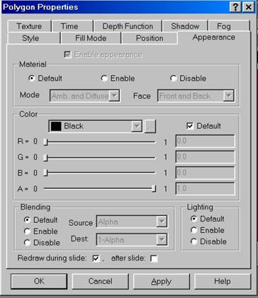
Lighting can be controlled by sliders and can be changed using edit boxes. It is convenient to deal with the RGBA components varying from 0 to 1. Edit fields can accept not only numerical values but also simple mathematical expressions which can involve project variables. There is also reserved time variable “t” to indicate time dependence. If player is running, it computes all object properties at given time moment “t” so several interesting effects like time-depending coloring can be reached. For example, to reach the effect of object disappearance set the Alpha component of color to “cos(t)*cos(t)” so that at t=0, it is equal to 1, while at any t = n*pi, it is equal to 0. This is full transparency. Press player button to see, that the object will appear and disappear with time.
Blending effect is also present. If enabled, it blends the incoming RGBA color values with the values in the color buffers. Pixels can be drawn using a function that blends the incoming (source) RGBA values with the RGBA values that are already in the frame buffer (the destination values). When enabled, the operation of blending is defined. The source factor parameter specifies which of methods is used to scale the source color components. The destination factor parameter specifies which of methods is used to scale the destination color components. For example, transparency is best implemented using ALPHA, 1-ALPHA. Not all combinations are possible here, see OpenGL manual for more detailed discussion.
A.2 Shadows of Objects
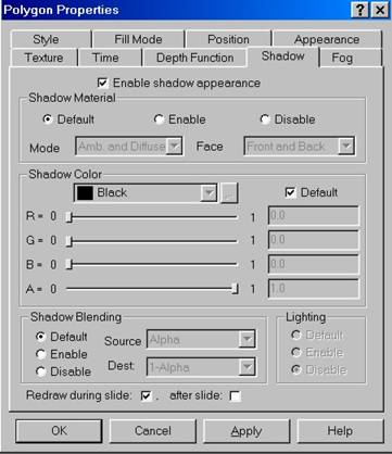 Object
shadows are treated in the same way as objects themselves. Therefore, settings
for shadow appearance are very similar to the settings of object appearance.
Several remarks are in order however. First you will need to create a special
object called a scene wall. Scene walls define the planes where objects are
drawn in a flattened form thus imitating the shadows. Second, you can switch on
or off shadow appearance, so that the scene walls either reflect shadows of the
given object coming from all light sources or not. For example, making shadows
of graph axis may not be desired for the final scene. Third, shadow surfaces do
not reflect light, so that lighting option is disabled by definition. Therefore
shadows appear with the constant color. However, a cool effect can be reached
by making semitransparent shadows (by changing Alpha components of the shadow
color). For textured scene walls, the effect looks very realistic when the
actual texture is seen through the shadows. You can also use simple
mathematical expressions and not only numerical values in the edit fields of
the color properties within Shadow property pages.
Object
shadows are treated in the same way as objects themselves. Therefore, settings
for shadow appearance are very similar to the settings of object appearance.
Several remarks are in order however. First you will need to create a special
object called a scene wall. Scene walls define the planes where objects are
drawn in a flattened form thus imitating the shadows. Second, you can switch on
or off shadow appearance, so that the scene walls either reflect shadows of the
given object coming from all light sources or not. For example, making shadows
of graph axis may not be desired for the final scene. Third, shadow surfaces do
not reflect light, so that lighting option is disabled by definition. Therefore
shadows appear with the constant color. However, a cool effect can be reached
by making semitransparent shadows (by changing Alpha components of the shadow
color). For textured scene walls, the effect looks very realistic when the
actual texture is seen through the shadows. You can also use simple
mathematical expressions and not only numerical values in the edit fields of
the color properties within Shadow property pages.
A.3 Scene Coordinate System and Projections
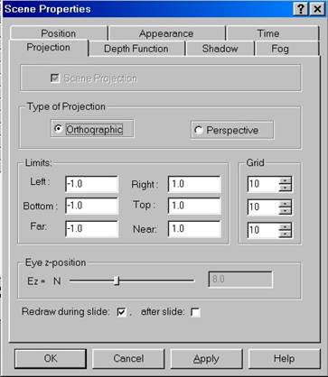 Objects
coordinates on the scene are given with respect to the Scene coordinate system
which represents a cube centered at the center of the Window and spans from –1
to 1 for left right direction, from –1 to 1 from bottom to top direction and
from –1 to 1 from far to near direction. Thus the object with coordinates
(0,0,0) will be exactly at the center of the Scene.
Objects
coordinates on the scene are given with respect to the Scene coordinate system
which represents a cube centered at the center of the Window and spans from –1
to 1 for left right direction, from –1 to 1 from bottom to top direction and
from –1 to 1 from far to near direction. Thus the object with coordinates
(0,0,0) will be exactly at the center of the Scene.
Since the scene and its objects are projected onto the screen plane we can deal with two kinds of projections: orthographic and perspective ones. Orthographic or parallel projections just flatten the objects with respect its z-component, therefore they look undistorted on the screen. If we consider screen coordinate system given by x,y axes, orthographic projection from the scene coordinates of any point (x,y,z) would just be its (x,y) components with respect to the screen coordinates. Perspective projections are designed to bring a 3D look to the objects so that when projecting onto the screen, x,y components of the objects in the screen coordinates take into account not only x,y components of the object in 3D scene coordinate (like with orthographic projections) but also its z-component.
How precisely we want to use a perspective projection depends on the eye coordinate which is given with respect to the far-near scene axis (axis perpendicular to the screen).
You can select either orthographic or perspective projection of the scene using Projection property page for the scene. Note that object tracking, i.e object selection with the mouse clicks is only allowed when using orthographic projections since the layout of the objects is undistorted here.
Use orthographic projections to build the scene and to layout all objects. Use perspective projections to bring to your scenes natural 3D look when the whole scene is composed.
A.4 Position of Objects
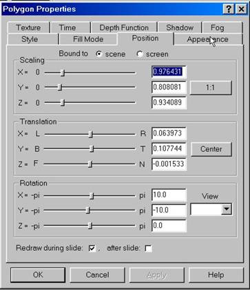 Object
position on the scene is one of its key properties. It is controlled by both Position
property page and Time property page. To start the discussion, we
introduce the coordinate system of the whole scene, which is given by three
axes. The first axis runs from left to right and is refereed as x-axis. The
limits are from –1 to 1. The second axis is y-axis that runs from bottom of the
screen to its top and we call it y-axis. The limits are from –1 to 1. The third
axis runs from far to near and it is called z-axis. The limits are again from
–1 to 1. Now as soon as coordinate system is given, all objects positions can
be given within these coordinates. We distinguish scaling, center position, and
rotations for all objects on the scene. By default, object with the scaling
along x,y,z = 1,1,1, centered at (0,0,0) and not rotated will be described by
the bounding cube at the center of scene with the sizes 1,1,1 so that it fills
exactly half of the scene at each direction, and therefore has a volume of 1/8
of the scene. We also distinguish static positions for the objects and the
dynamic positions. The latter ones are computed at every time moment “t” if the
scene player is running. This property page deals with only static object positions.
Another property page “time”
deals with the time-dependent components.
Object
position on the scene is one of its key properties. It is controlled by both Position
property page and Time property page. To start the discussion, we
introduce the coordinate system of the whole scene, which is given by three
axes. The first axis runs from left to right and is refereed as x-axis. The
limits are from –1 to 1. The second axis is y-axis that runs from bottom of the
screen to its top and we call it y-axis. The limits are from –1 to 1. The third
axis runs from far to near and it is called z-axis. The limits are again from
–1 to 1. Now as soon as coordinate system is given, all objects positions can
be given within these coordinates. We distinguish scaling, center position, and
rotations for all objects on the scene. By default, object with the scaling
along x,y,z = 1,1,1, centered at (0,0,0) and not rotated will be described by
the bounding cube at the center of scene with the sizes 1,1,1 so that it fills
exactly half of the scene at each direction, and therefore has a volume of 1/8
of the scene. We also distinguish static positions for the objects and the
dynamic positions. The latter ones are computed at every time moment “t” if the
scene player is running. This property page deals with only static object positions.
Another property page “time”
deals with the time-dependent components.
We keep in mind that the final object position is a combination of its static and dynamic components. This works slightly differently for scaling, center position, and rotational elements. For scaling, the final scaling position at time moment t is computed as a product of its static scaling factor which is set up here and the time dependent factor which is set up by the time property page. For displacements from the center and for rotations the final value is a sum of static and dynamic components.
By default, time dependent settings for scaling are 1,1,1, for center are 0,0,0, and for rotational angles are 0,0,0. Therefore, default object position is entirely controlled by the static components. In summary, when constructing the object, keep in mind that you can apply scaling, displacements, and rotational operations easily, therefore coordinate system for the object itself can be chosen in most appropriate way.
A little more complication will arrive when we say that the scene itself is a kind of object and can therefore have its own scaling factors, displacements and rotations. Therefore if we rotate or scale the whole scene, we have to say whether the objects will follow these distortions or not. We distinguish objects that are either bounded to the scene or to the screen. If the object is bounded to the scene coordinate system its position is with respect to the scene position, therefore rotation of the scene will rotate the object. If, on the other hand, the object is bounded to the screen, changing the scene properties will not affect position of the object. By default all objects are bounded to the scene. For example, setting time-depending scene rotation will rotate all objects as well.
A.5 Time-Dependent Position.
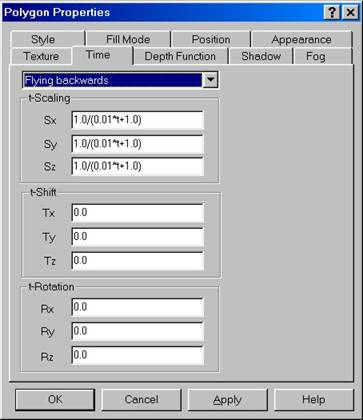 To
discuss time dependent position please first read the discussion of objects
positions in general. (See Position of Objects). Time dependency is
controlled by Time property page. If we would like to achieve “flying
effect” for the object on the scene we need to change its coordinates as a
function of time. Then, when we render the scene by the player, all properties
are computed for given time moment “t” and we reach several coolest effects. We
specified several obvious functions that will describe such effects. As example
consider “flying out” and “flying in” effects. If we change object scale from 1
to zero by 1/(1+t) or similar function which is 1 at t=0 and 0 at t=infinity,
the object will decrease its dimension with time so that it is “flying away”.
Similarly, if we say that it scales from 0 to 1 as for example given by the
formula like 1-1/(1+t). it will obviously “fly in”. You may also use project
variables when building the formulae that sometimes gives the convenience of
changing the variable value in one place instead of modifying many property
pages of various objects.
To
discuss time dependent position please first read the discussion of objects
positions in general. (See Position of Objects). Time dependency is
controlled by Time property page. If we would like to achieve “flying
effect” for the object on the scene we need to change its coordinates as a
function of time. Then, when we render the scene by the player, all properties
are computed for given time moment “t” and we reach several coolest effects. We
specified several obvious functions that will describe such effects. As example
consider “flying out” and “flying in” effects. If we change object scale from 1
to zero by 1/(1+t) or similar function which is 1 at t=0 and 0 at t=infinity,
the object will decrease its dimension with time so that it is “flying away”.
Similarly, if we say that it scales from 0 to 1 as for example given by the
formula like 1-1/(1+t). it will obviously “fly in”. You may also use project
variables when building the formulae that sometimes gives the convenience of
changing the variable value in one place instead of modifying many property
pages of various objects.
A.6 Testing Depth and Transparency for Objects
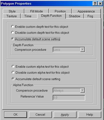 These
settings are implemented for completeness but you in fact will rarely want to
change them to. They are controlled by Depth Function property page.
These
settings are implemented for completeness but you in fact will rarely want to
change them to. They are controlled by Depth Function property page.
Since objects are seen in three dimensional space, some of the objects are closer than the other. When overlap occurs, the program should compute which part of the object is seen and which part of it is covered by other objects. This procedure is called depth test. Depth test is made by comparison z-components of the object position (z-axis is equivalent to far-near axis of the screen coordinate system). Depending on actual z-values for two objects, the program decides whether test is passed or not from the depth function selected within this property page. Finally, you can disable depth comparison procedure, so that all objects will be drawn.
Another kind of test is called alpha-testing and is related to object transparency. You may set a certain cutoff value for the alpha-component of the object color so that if the alpha test is passed, the object is seen on the scene while if the object alpha value does not pass the comparison procedure, the object is not seen on the scene. The cutoff value is set within this property page and the desired comparison procedure can be selected.
A.7 Textures
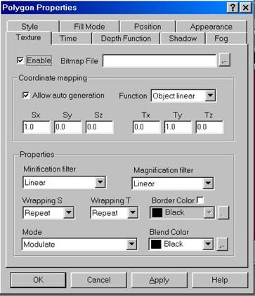 Texturing
is one of the most excited features of the 3D graphics. Texture mapping is a
technique that applies an image onto object's surface as if the image were a
decal or cellophane shrink-wrap. The image is created in texture space, with an
(s, t) coordinate system (only s for 1D objects). A texture is a
one- or two-dimensional image and a set of parameters that determine how
samples are derived from the image. Controlling the object texturing is done by
Texture property pages.
Texturing
is one of the most excited features of the 3D graphics. Texture mapping is a
technique that applies an image onto object's surface as if the image were a
decal or cellophane shrink-wrap. The image is created in texture space, with an
(s, t) coordinate system (only s for 1D objects). A texture is a
one- or two-dimensional image and a set of parameters that determine how
samples are derived from the image. Controlling the object texturing is done by
Texture property pages.
To allow texturing of your object surface, you will need a standard Windows bitmap file (extension .bmp) that contains your image. A special comment should be said about image dimensions. Since we allow to scale our objects, the images should be scaled as well. Scaling images procedure requires that all images have their sizes (width and height) to be representable in terms of powers of 2, i.e 2^k with k to be some integer. Since image may be smaller that the object surface, we can either repeat or clamp the image onto the surface. In the repeating procedure, we can allow one-pixel border between images to occur. So, if border is allowed, the sizes of the images should be representable as 2^k + 1. If your image does not have proper dimensions, the program will cut its sizes to the nearest 2^k representability. The corresponding message will warn you if this needs to happen.
Another important thing to discuss is how actual image coordinates are mapped into object surface. This procedure is called texture mapping. For 2D case, image has (s,t) coordinates varied from 0 to 1 (image start to image end). Two procedures are implemented within the program: manual texture mapping and automatic texture mapping. For simple objects like polygons (cubes) you may directly associate every vertex coordinate with a particular image coordinate so that you are sure that your image is placed on the surface exactly in a way you would like. For complicated objects this requires a lot of work and, therefore, automatic mapping procedure is more preferable. Three automatic chooses are available: OBJECT LINEAR, EYE LINEAR, AND SPHERE MAPPING. The best way to figure out which way is nice is to try out. Note that since texture coordinates are generated by some function, called autogeneration function, you can change the coefficients of these functions, thus having at least some control on automapping procedure. If you switch off automapping, it is assumed that the texture coordinates are explicitly given.
You have choices to select which procedure will be used to throw away pixels when you scale your images. The texture minifying function is used whenever the pixel being textured maps to an area greater than one texture element. It uses the nearest one (NEAREST) or nearest four (LINEAR) texture elements to compute the texture value. The texture magnification function is used when the pixel being textured maps to an area less than or equal to one texture element. This sets the texture magnification function to either NEAREST or LINEAR.
Also, you can control the wrap parameter for texture coordinates to either CLAMP or REPEAT. CLAMP causes coordinates to be clamped to the range [0,1] and is useful for preventing wrapping artifacts when mapping a single image onto an object. REPEAT causes the integer part of the s coordinate to be ignored; OpenGL uses only the fractional part, thereby creating a repeating pattern. Border texture elements are accessed only if wrapping is set to CLAMP.
Discussion of 1D texturing is very similar but you do not have access to controls of the second dimension.
A.8 Fog Effect
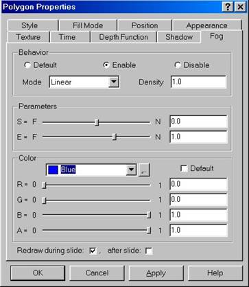 Fog
is a really cool effect that is best seen by trying out on some example. Create
a ball at the center of the scene, light it, enable color of the ball, put to
green or similar, and start changing near (S) and far (E) distances of the fog
equation, the controls appeared within Fog property page. You should see
how properties of the ball surface would be changed by this effect. The fog
distance and density determine how much fog color is mixed in. By default, fog
is applied at all depths from 0.0 to 1.0. The start and end parameters restrict
the range of depth values used for fog calculations. This range is typically
used to more accurately model fog density when the immediate area in front of
the viewer is not covered or for prematurly “fogging out” the scene before the
far plane is reached.
Fog
is a really cool effect that is best seen by trying out on some example. Create
a ball at the center of the scene, light it, enable color of the ball, put to
green or similar, and start changing near (S) and far (E) distances of the fog
equation, the controls appeared within Fog property page. You should see
how properties of the ball surface would be changed by this effect. The fog
distance and density determine how much fog color is mixed in. By default, fog
is applied at all depths from 0.0 to 1.0. The start and end parameters restrict
the range of depth values used for fog calculations. This range is typically
used to more accurately model fog density when the immediate area in front of
the viewer is not covered or for prematurly “fogging out” the scene before the
far plane is reached.
B.1 Styles for Line Strip Objects
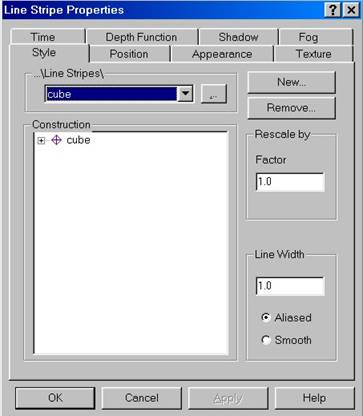 When
line strip object is created it is a simple cube by default. However, any
object represented by a set of connected lines (line strips) can be drawn by
the program. Style property page for line strip objects allows the
construction of any line strip. The line strips are represented by a set of
lines, each of those is given by a set of vertexes (points).
When
line strip object is created it is a simple cube by default. However, any
object represented by a set of connected lines (line strips) can be drawn by
the program. Style property page for line strip objects allows the
construction of any line strip. The line strips are represented by a set of
lines, each of those is given by a set of vertexes (points).
To define every lines trip, a set of vertexes should be described. The vertex points are given by the x,y,z coordinates with respect to the Scene coordinate system. Also RGBA color values can be associated with every vertex point and the linear texture coordinate s. The corresponding tree control exists at the Style Property pages which allows creation/editing of such objects. Use right-mouse-button pop-up menus to add/remove vertexes for line strip objects.
Color values associated with every vertex will produce given line colored according to interpolations between colors set for every two vertexes.
Texture coordinate is used in connections with Texture Properties of the objects. How given texture is mapped to the line can be set using linear texture coordinate t (t=0 – beginning of the image, t =1 – end of the image) associated with every vertex point.
Every line strip is stored in the formatted ASCII file so that in principle such files can be created/edited externally. Each time the line strip object is selected, the program reads the file from the Line Strips database. Every time Apply button is pressed the program stores the given line strip object back to the file.
When line strip object is created it is a simple cube by default. The program read cube.lin file from the Line Strips database.
The necessary input for lines trip objects are only the vertex coordinates. RGBA colors and texture coordinates are optional. When constructing the line strips using tree control, use the word auto to show that the current value will be computed automatically. When editing the corresponding ASCII files you may skip vertex colors and textures values at all, or use -1-1-1-1 for colors, and -1 for textures to indicate that these are computed automatically. Refer to the examples of cube and tetrahedron that exist in the Line Strips folder within the directory the program is installed.
Instead of creating line strip objects manually you may convert every 3D Curve drawn within the Graph layer into the line strip object. Use pop-up menu of the 3D curve icon within the Object Explorer and use command Export As Object to make this conversion. This will create a line strip object within the Line Strips Database.
B.2 Styles for Polygonal Objects
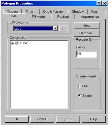 When
polygonal object is created it is a simple cube by default. However, any object
represented by a set of polygons can be drawn by the program. Style property
page for polygonal objects allows the construction of any polygon. The
polygons are represented by a set of faces, each of those is given by a set of
vertexes (points).
When
polygonal object is created it is a simple cube by default. However, any object
represented by a set of polygons can be drawn by the program. Style property
page for polygonal objects allows the construction of any polygon. The
polygons are represented by a set of faces, each of those is given by a set of
vertexes (points).
To define every face, a set of vertexes should be described. The vertex points are given by x,y,z coordinates with respect to the Scene coordinate system. Also RGBA color values can be associated with every vertex point and the texture coordinates t,s. The corresponding tree control exists at the Style Propery pages that allows creation/editing of such objects. Use right-mouse-button pop-up menus to add/remove vertexes and faces from your polygonal objects.
Color values associated with every vertex will produce given polygonal face colored according to interpolations between all colors set for all face vertexes.
Texture coordinates are used in connections with Texture Properties of the objects. How given texture is mapped to the polygon can be set using texture coordinates t,s (t,s=0 – beginning of the image, t,s =1 – end of the image) associated with every vertex point.
Normals to the polygonal objects can be defined either to every face of the polygon or to every vertex in the polygon. To produce flat-cut surfaces choose normals to every polygonal face. To produce smooth surface objects choose normals to every polygonal vertex. This difference is readily seen between cube and sphere. For the cube, normal to every cube face is selected, while for the sphere normal to every vertex is selected so that spherical objects look much smoother.
Every polygon is stored in the formatted ASCII file so that in principle such files can be created/edited externally. Each time polygonal object is selected, the program reads the file from the Polygons database. Every time Apply button is pressed the program stores the given polygonal object back to the file.
When polygonal object is created it is a simple cube by default. The program read cube.pol file from the polygons database.
The necessary input for polygonal objects is only the vertex coordinates. Normals, RGBA colors and texture coordinates are optional. When constructing the polygons using tree control, use the word auto to show that the current value will be computed automatically. When editing the corresponding ASCII files you may not indicate the vertex normals, colors and textures values at all, or use 0,0,0 for normals, -1-1-1-1 for colors, and -1-1 for textures to indicate these are computed automatically. Refer to the examples of cube and tetrahedron that exists in the Polygons folder within the directory the program is installed.
Instead of creating polygonal objects manually you may convert every surface drawn within the Graph layers into polygonal object. Use pop-up menu of the surface icon within the Object Explorer and use command Export As Object to make this conversion. This will create a polygonal object within the Polygons Database. Note that the way the normals are chosen to the surface will be stored and you will have no chance to use another normal generation algorithm after polygonal object is created and stored. If surface is represented by several sheets use the tree control related to surface properties to show/hide any of these sheets before storing the objects. Only surface sheets that are currently shown will be converted into polygonal object.
A special object called Wall exists for the scene. Walls are just planes where objects shadows are drawn. Since Wall is constructed as a polygon, the same property page is applied to this object. See also the discussion of shadows appearance
B.3 Filling Modes for Polygonal Objects
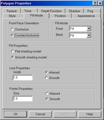 Surfaces
of polygonal objects can be customized using Fill Mode property pages.
These property pages allow define front and back faces of the surfaces, as well
as the way front and back faces are drawn (either as filled polygons, line
stripes or simple points).
Surfaces
of polygonal objects can be customized using Fill Mode property pages.
These property pages allow define front and back faces of the surfaces, as well
as the way front and back faces are drawn (either as filled polygons, line
stripes or simple points).
B.4 Styles for Quadric Objects
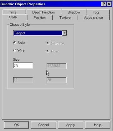 Quadric
objects are drawn using OpenGL utility library. Several popular objects like
spheres and cylinders can be directly drawn using Style property pages
applicable to quadric objects. There is no need to construct polygons for such
objects. By default spheres are created for quadric objects but they can be
replaced by any other object available in the library with help of the Style
property page.
Quadric
objects are drawn using OpenGL utility library. Several popular objects like
spheres and cylinders can be directly drawn using Style property pages
applicable to quadric objects. There is no need to construct polygons for such
objects. By default spheres are created for quadric objects but they can be
replaced by any other object available in the library with help of the Style
property page.
B.5 Changing Graph Style
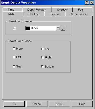 Despite
graphs are complicated objects that consist of layers, axes, surfaces, you may
want to customize the graph frame appearance itself. To do it use Style
property page when navigating graph object properties. The frame for the
graph object can be toggled on/off and the planes of the bounding cube can be
shown. You may customize their appearance and color using other property pages
for the graph objects. However, this set of properties does not allow you to
access to properties of the layers, axis, and surfaces that may be associated
with given graph object. To find properties for the axis and surfaces navigate
content of the graph via Project Explorer.
Despite
graphs are complicated objects that consist of layers, axes, surfaces, you may
want to customize the graph frame appearance itself. To do it use Style
property page when navigating graph object properties. The frame for the
graph object can be toggled on/off and the planes of the bounding cube can be
shown. You may customize their appearance and color using other property pages
for the graph objects. However, this set of properties does not allow you to
access to properties of the layers, axis, and surfaces that may be associated
with given graph object. To find properties for the axis and surfaces navigate
content of the graph via Project Explorer.
B.6 Styles for Scene Objects.
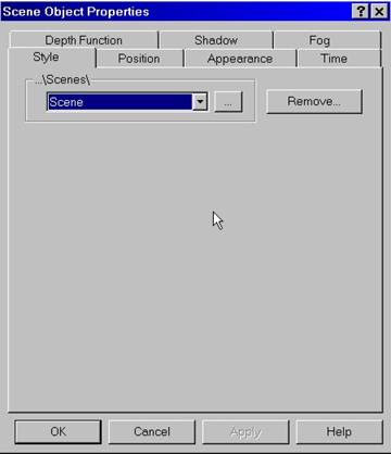 This
is one of the most exciting features in 3D modeling. Once you constructed your
scene with complicated layout of various objects, the obvious question is
whether we can store the entire scene as a single object and then use it as a
building block in another, more complicated scene. Conversion of scene into the
object is possible using Save As Object command within the Scene
menu. Once you converted your scene into the object it will be stored in the
Scene Database. In order to create the scene object from the database select Scene
Tool from the Scene Toolbar or use Set Mode -> Scene
command within the Scene menu. Create a scene object. By default scene.scn file will be read from
the Scene Database that contains the default scene. After that the Style
property page appears which allows you to select desired scene object from
the database.
This
is one of the most exciting features in 3D modeling. Once you constructed your
scene with complicated layout of various objects, the obvious question is
whether we can store the entire scene as a single object and then use it as a
building block in another, more complicated scene. Conversion of scene into the
object is possible using Save As Object command within the Scene
menu. Once you converted your scene into the object it will be stored in the
Scene Database. In order to create the scene object from the database select Scene
Tool from the Scene Toolbar or use Set Mode -> Scene
command within the Scene menu. Create a scene object. By default scene.scn file will be read from
the Scene Database that contains the default scene. After that the Style
property page appears which allows you to select desired scene object from
the database.
A special note should be said about light sources and walls. We would like to have scene objects lightened according to the given set of light sources and produce shadows onto given set of walls. Therefore scene objects do not contain either light sources or wall objects. In other words, when the program stores the scene object it skips all presented light sources and walls.
B.7 3D Text and its Style
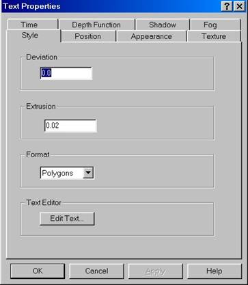 Use
Text tool to add text to the scene. To customize text appearance use text Style
Property Page. The fonts for labels are extracted from those installed on
your computer. You may give a 3D look to your labels. Give a finite value to extrusion
property. Having been treated as objects, labels have surfaces, therefore they
are colored and lightened. To change fonts, text size and color use text
editor.
Use
Text tool to add text to the scene. To customize text appearance use text Style
Property Page. The fonts for labels are extracted from those installed on
your computer. You may give a 3D look to your labels. Give a finite value to extrusion
property. Having been treated as objects, labels have surfaces, therefore they
are colored and lightened. To change fonts, text size and color use text
editor.
The program approximates glyph outlines by subdividing the quadratic B-spline curves of the outline into line segments, until the distance between the outline and the interpolated midpoint is within the value specified by deviation. This is the final format used when format is LINES. When you specify LINES, the glyphs created don't contain any normals; thus lighting doesn't work properly. To get the correct lighting use format POLYGONS. When you specify format as POLYGONS the outlines are further tessellated into separate triangles, triangle fans, triangle strips, or quadrilateral strips to create the surface of each glyph.
C.1 Cartesian 2D Axis Orientation and Type
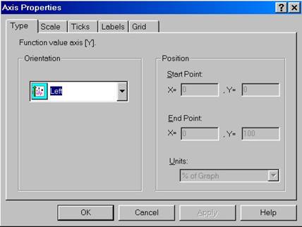 Cartesian
axes can be oriented either vertically or horizontally. This is controlled by
axis Type property page. Some care should be taken when axis changes its
orientation from horizontal to vertical or vice versa. Since the layer is
characterized by two sets of principal axes perpendicular to each other, both
principal axes should change their orientation spontaneously. Cartesian axes
are not necessarily positioned into bottom/top/left/right positions. They can
be generally vertical or horizontal. To select a vertical position use either
units of percents of graph or current scale of perpendicular axis. For example
bottom axis corresponds to 0% position in the graph scale and top axis would
correspond to 100% in the graph scale.
Cartesian
axes can be oriented either vertically or horizontally. This is controlled by
axis Type property page. Some care should be taken when axis changes its
orientation from horizontal to vertical or vice versa. Since the layer is
characterized by two sets of principal axes perpendicular to each other, both
principal axes should change their orientation spontaneously. Cartesian axes
are not necessarily positioned into bottom/top/left/right positions. They can
be generally vertical or horizontal. To select a vertical position use either
units of percents of graph or current scale of perpendicular axis. For example
bottom axis corresponds to 0% position in the graph scale and top axis would
correspond to 100% in the graph scale.
C.2 Polar 2D Axis Orientation and Type
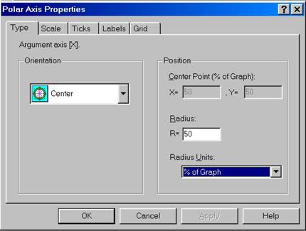 In
most cases polar axis is oriented at the center of the graph. To shift it away
from the center use polar axis Type property page.
In
most cases polar axis is oriented at the center of the graph. To shift it away
from the center use polar axis Type property page.
C.3 Radial 2D Axis Orientation and Type
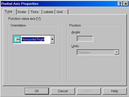 Radial
axis at polar graphs originates from the center of the graph and ends up at the
radius as given by the polar axis. The orientation of the radial axis is set up
in terms of radial axis Type property page.
Radial
axis at polar graphs originates from the center of the graph and ends up at the
radius as given by the polar axis. The orientation of the radial axis is set up
in terms of radial axis Type property page.
C.4 Cartesian 2D Axis Scale
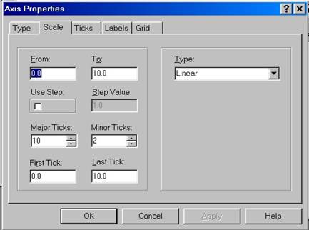 Which
value is associated with axis start and which is associated with its end is set
up by the axis Scale Property Page. To divide the axis into a set of
equidistant intervals you may either use a fixed step or the number of
divisions. Both of them can be customized using these property pages. Small
ticks will appear on the axis to indicate the number of intervals. Each
interval can be further subdivided by a set of subintervals. We distinguish
major ticks and minor ticks in this way. Ticks size and direction can be
further customized using Ticks property pages.
Which
value is associated with axis start and which is associated with its end is set
up by the axis Scale Property Page. To divide the axis into a set of
equidistant intervals you may either use a fixed step or the number of
divisions. Both of them can be customized using these property pages. Small
ticks will appear on the axis to indicate the number of intervals. Each
interval can be further subdivided by a set of subintervals. We distinguish
major ticks and minor ticks in this way. Ticks size and direction can be
further customized using Ticks property pages.
Finally, we use linear axis scale only and logarithmic scale will be implemented in the future releases.
C.5 Polar 2D Axis Scale
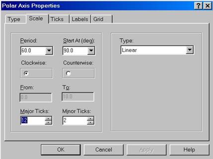 Since
polar axis is designed to measure the angle, scale for the polar axis is given
from 0 to 360 degrees in most cases. We however may choose either clockwise or
counterclockwise orientation here. To divide the axis into a set of equidistant
intervals you may either use a fixed step or the number of divisions. Both of
them can be customized within this property page. Small ticks will appear on
the axis to indicate the number of intervals. Each interval can be further
subdivided by a set of subintervals. We distinguish major ticks and minor ticks
in this way. Ticks size and direction can be further customized using Ticks
property pages.
Since
polar axis is designed to measure the angle, scale for the polar axis is given
from 0 to 360 degrees in most cases. We however may choose either clockwise or
counterclockwise orientation here. To divide the axis into a set of equidistant
intervals you may either use a fixed step or the number of divisions. Both of
them can be customized within this property page. Small ticks will appear on
the axis to indicate the number of intervals. Each interval can be further
subdivided by a set of subintervals. We distinguish major ticks and minor ticks
in this way. Ticks size and direction can be further customized using Ticks
property pages.
Finally, we use linear axis scale for angular axis types.
C.6 2D Axis Ticks
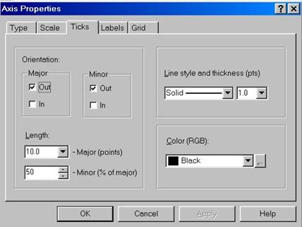 Ticks
are small lines that are perpendicular to axis direction and can be controlled
by Ticks property pages. Usually you also put labels at the end of every
tick which are controlled by Labels property pages
Ticks
are small lines that are perpendicular to axis direction and can be controlled
by Ticks property pages. Usually you also put labels at the end of every
tick which are controlled by Labels property pages
You can choose to have major ticks that divide axis onto a set of intervals and minor ticks that subdivide every interval onto a set of subintervals.
C.7 2D Axis Labels
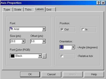 To
customize axis labels use Labels Property Page. The fonts for labels are
extracted from those installed on your computer. You may change the color,
offset, and size of the labels. All distances are given in points (one inch is
72 points)
To
customize axis labels use Labels Property Page. The fonts for labels are
extracted from those installed on your computer. You may change the color,
offset, and size of the labels. All distances are given in points (one inch is
72 points)
C.8 Showing Grid
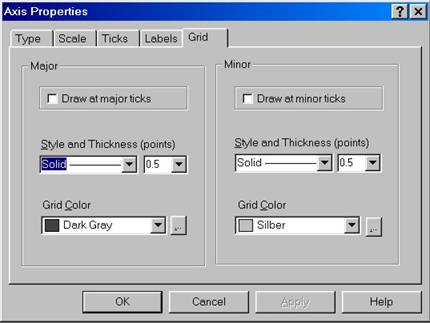 To
show grid lines on your graph use Grid property page. Grid lines can be
drawn parallel to every major tick and to every minor tick. You may select
various colors for grid lines, different for major grid lines and for minor
grid lines. Note that since the grid is given by the property of the axis, i.e.
a set of lines perpendicular to the axis, you will need to customize both
argument and function axis to have a square grid appeared on your graph.
To
show grid lines on your graph use Grid property page. Grid lines can be
drawn parallel to every major tick and to every minor tick. You may select
various colors for grid lines, different for major grid lines and for minor
grid lines. Note that since the grid is given by the property of the axis, i.e.
a set of lines perpendicular to the axis, you will need to customize both
argument and function axis to have a square grid appeared on your graph.
C.9 3D Axis Orientation and Type
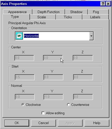 To
orient axis in 3D space, use Type property pages. In general we
distinguish principal axes and auxiliary axes. Principal axes set up a
coordinate system for the layer therefore they should represent an orthogonal
system. Auxiliary axes are used for convenience only and do not affect the
layer coordinates.
To
orient axis in 3D space, use Type property pages. In general we
distinguish principal axes and auxiliary axes. Principal axes set up a
coordinate system for the layer therefore they should represent an orthogonal
system. Auxiliary axes are used for convenience only and do not affect the
layer coordinates.
Due to this orthogonality problem 3D axis orientation has to be done with care. For Cartesian layers, we have 3 possible orientations in general. For polar systems we have one radial axis that originates at the center of the sphere and we also have two angular axes, for phi and theta, whose planes must be orthogonal to each other. For cylinder coordinates we have one radial axis and one angular axis plus we have a vertical axis.
It is now important to note
that the scene coordinate system is given by Cartesian axes which are
left-right, bottom-top, and far-near and are refereed ever
In general, you will not be allowed to change axis orientation, and customization is reduced to parallel shifts of the axis within the graph. However, for auxiliary axis any orientation does not affects the properties of the layer and you can choose to position it at any convenient location.
C.10 3D Axis Scale
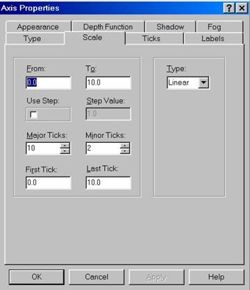 Which
value is associated with axis start and which is associated with its end is set
up by the axis Scale Property Page. To divide the axis into a set of
equidistant intervals you may either use a fixed step or the number of
divisions. Both of them can be customized using these property pages. Small
ticks will appear on the axis to indicate the number of intervals. Each
interval can be further subdivided by a set of subintervals. We distinguish
major ticks and minor ticks in this way. Ticks size and direction can be further
customized using Ticks property pages.
Which
value is associated with axis start and which is associated with its end is set
up by the axis Scale Property Page. To divide the axis into a set of
equidistant intervals you may either use a fixed step or the number of
divisions. Both of them can be customized using these property pages. Small
ticks will appear on the axis to indicate the number of intervals. Each
interval can be further subdivided by a set of subintervals. We distinguish
major ticks and minor ticks in this way. Ticks size and direction can be further
customized using Ticks property pages.
Finally, we use linear axis scale only and logarithmic scale will be implemented in the future releases.
C.11 3D Axis Ticks
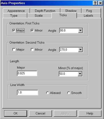 Ticks
are small lines that are perpendicular to axis direction and can be controlled
by Ticks property pages. . Usually you also put labels at the end of
every tick that are controlled by Labels property pages.
Ticks
are small lines that are perpendicular to axis direction and can be controlled
by Ticks property pages. . Usually you also put labels at the end of
every tick that are controlled by Labels property pages.
Two sets of ticks can be produced on 3D axis. You can also choose to have major ticks that divide axis onto a set of intervals and minor ticks that subdivide every interval onto a set of subintervals. To customize ticks drawing, select desired line width and smoothing procedure. Ticks color and lighting properties are the same as for the whole axis and can be found in the other property pages of the axis object.
C.12 3D Axis Labels
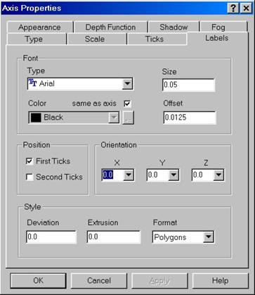 To
customize 3D axis labels use Labels Property Page. The fonts for labels
are extracted from those installed on your computer. You may change the color,
offset, and size of the labels. You may
have two sets of ticks on your 3D axis, so that you may put labels near each
set of ticks. All distances used are related to the scene coordinate system
described within Scene Projection. Normally, the dimension of the
scene along x,y,z direction is 2,2,2 (-1 to 1, -1 to 1, -1 to 1) so that the
typical label dimension maybe 0.01 or so. Try out several sizes to find out the
best looking one.
To
customize 3D axis labels use Labels Property Page. The fonts for labels
are extracted from those installed on your computer. You may change the color,
offset, and size of the labels. You may
have two sets of ticks on your 3D axis, so that you may put labels near each
set of ticks. All distances used are related to the scene coordinate system
described within Scene Projection. Normally, the dimension of the
scene along x,y,z direction is 2,2,2 (-1 to 1, -1 to 1, -1 to 1) so that the
typical label dimension maybe 0.01 or so. Try out several sizes to find out the
best looking one.
You may also give a 3D look to your labels. Give a finite value to extrusion property. Having been treated as objects, labels have surfaces, therefore they are colored and lightened. These properties are controlled by the axis settings and the labels encapsulate them.
D.1 2D Curves: General Properties
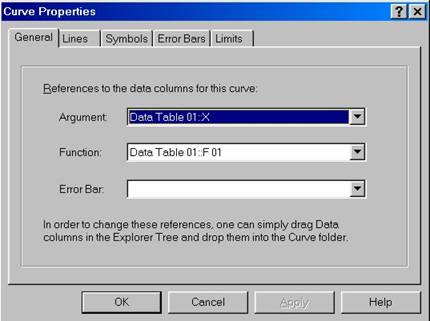 Curves
are the objects that are connected to the data columns. Two types of data
columns define the curve: argument column and the function column. Thus, to
plot function f(x) you will need to create the column X (associated with the
argument) and the column F (associated with the function values). Additionally
curves can be linked to error bar columns, this gives the possibility to plot
error bars or widen the curves proportionally to the given function.
Curves
are the objects that are connected to the data columns. Two types of data
columns define the curve: argument column and the function column. Thus, to
plot function f(x) you will need to create the column X (associated with the
argument) and the column F (associated with the function values). Additionally
curves can be linked to error bar columns, this gives the possibility to plot
error bars or widen the curves proportionally to the given function.
General property page shows link between columns in the data tables and the curve objects. There are several ways to set up such links. One way is to drag the data column item on the Explorer Tree and drop it within the layer folder. Curve object will be created automatically in this way. If you drag a function column, the program will look for the argument column in the given data table and will make automatic connection of both argument and function to the curve object. If you drag only the argument column, only connection to the argument will be established. Error bar columns should be linked to the curves separately. Another way to make a link is to create empty curve object using the pop-up menu within the layer folder. After empty curve object is created, call for properties dialog box and select General property page. The combo boxes allow you to make connections between the curve and the argument, function, and optionally error bar columns. Once both links to argument and function columns are established the curve should appear within the graph layer of a given plot page.
D.2 2D Curves Appearance
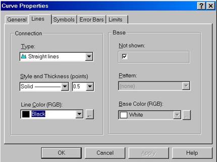 Curve
appearance within graph layers can be customized using Lines Property Page.
Desired connection style between points defining the curve can be chosen
together with the line width, color, curve base, etc.
Curve
appearance within graph layers can be customized using Lines Property Page.
Desired connection style between points defining the curve can be chosen
together with the line width, color, curve base, etc.
D.3 2D Curves Symbols
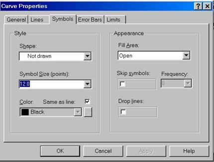 Symbols
can be placed on the original data points defining the curve. This is
controlled by Symbols property page. You have options to select desired
symbol style, size, color, how to fill the area inside the symbol, the
possibility to skip symbols with given frequency, and also drop lines from
every symbol to the argument axis.
Symbols
can be placed on the original data points defining the curve. This is
controlled by Symbols property page. You have options to select desired
symbol style, size, color, how to fill the area inside the symbol, the
possibility to skip symbols with given frequency, and also drop lines from
every symbol to the argument axis.
D.4 2D Curve Error Bars
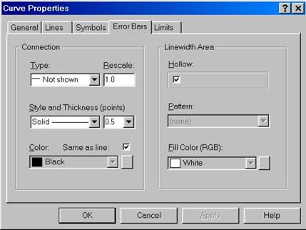 Error
Bars are important elements in the curve visualization analysis. Whether
experimental inaccuracy is known or an extra information should be associated
with every data points Error Bars property page offers a way to draw
this set of data on top of each curve. To accomplish this task, a column in the
data table should be created together with the argument column and the function
value column(s). The column should be associated with the ErrorBar. After
ErrorBar column exists, it should be connected to the curve that is drawn. You
may drag the error bar column item from the table tree and drop it into the
ErrorBar slot of the curve tree.
Error
Bars are important elements in the curve visualization analysis. Whether
experimental inaccuracy is known or an extra information should be associated
with every data points Error Bars property page offers a way to draw
this set of data on top of each curve. To accomplish this task, a column in the
data table should be created together with the argument column and the function
value column(s). The column should be associated with the ErrorBar. After
ErrorBar column exists, it should be connected to the curve that is drawn. You
may drag the error bar column item from the table tree and drop it into the
ErrorBar slot of the curve tree.
Two styles for the error bars are available, RESOLUTION, and LINEWIDTH. Resolution style is a classical error bar style which shows experimental inaccuracy of the given data point. Linewidth style widens the curve proportionally to the error bar function data so that the curve has a finite ‘’fatness’’. The latter effect may be important for eigenvalue problem analysis to show partial characters of the eigenvectors in each eigenvalue as well as for other problems. You have full customization possibilities of both error bar styles. Error bars can be also rescaled by a constant factor that is also directly controlled by this property page with no need to modify the original column data.
D.5 2D Curves Limits
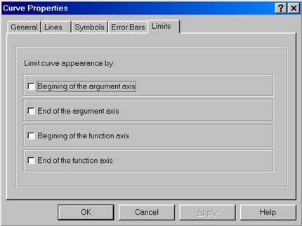 If
limits of the curve argument or function values are larger that the limits of
the axes within given graph layer, use Limits property page, to restrict
curve appearance exactly by the rectangular region defining the graph.
If
limits of the curve argument or function values are larger that the limits of
the axes within given graph layer, use Limits property page, to restrict
curve appearance exactly by the rectangular region defining the graph.
D.6 3D Curves & Surfaces: General
Properties
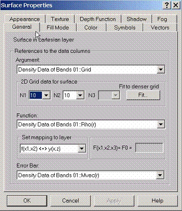 3D
Curves and Surfaces are the objects that are connected to the data columns.
This is very similar to the 2D curve objects. Two types of data columns define
the 3D curve or surface: argument column and the function column. Note here
that the argument column should contain a set of 2 or 3 data. To plot function
f(x1,x2) you will need a 2data argument column, and to draw the cross-section
f(x1,x2,x3)=f0, you will need to consider a 3data argument columns. Thus, to
plot function f(x1,x2) you will need to create the column X (associated with
the argument) which itself consists of two (sub)columns showing both values x1
and x2, You will also need to create the
column F associated with the function values. You may consider the possibility
to create a multidata column F (which consists of several (sub)columns). In
this way, the program will create a set of surfaces according to the number of
data in the function column. The advantage is that you can use only one set of
customization properties to visualize this set of surfaces. Additionally 3D
curves/surfaces can be linked to the error bar columns, which gives the
possibility to color these objects depending on the auxiliary function set up
by the error bar columns. Also a set of symbols can be drawn for the original
data points defining the surfaces with the size of the symbols scalable
according to the error bar column data.
3D
Curves and Surfaces are the objects that are connected to the data columns.
This is very similar to the 2D curve objects. Two types of data columns define
the 3D curve or surface: argument column and the function column. Note here
that the argument column should contain a set of 2 or 3 data. To plot function
f(x1,x2) you will need a 2data argument column, and to draw the cross-section
f(x1,x2,x3)=f0, you will need to consider a 3data argument columns. Thus, to
plot function f(x1,x2) you will need to create the column X (associated with
the argument) which itself consists of two (sub)columns showing both values x1
and x2, You will also need to create the
column F associated with the function values. You may consider the possibility
to create a multidata column F (which consists of several (sub)columns). In
this way, the program will create a set of surfaces according to the number of
data in the function column. The advantage is that you can use only one set of
customization properties to visualize this set of surfaces. Additionally 3D
curves/surfaces can be linked to the error bar columns, which gives the
possibility to color these objects depending on the auxiliary function set up
by the error bar columns. Also a set of symbols can be drawn for the original
data points defining the surfaces with the size of the symbols scalable
according to the error bar column data.
General property page shows link between columns in the data tables and the surface objects. There are several ways to set up such links. One way is to drag the data column item on the Explorer Tree and drop it within the layer folder. Surface object will be created automatically in this way. If you drag a function column, the program will look for the argument column in the given data table and will make automatic connection of both argument and function to the curve object. If you drag only the argument column, only connection to the argument will be established. Error bar columns should be linked to the surfaces separately. Another way to make a link is to create empty surface object using the pop-up menu within the layer folder. After empty surface object is created, call for properties dialog box and select General property page. The combo boxes allow you to make connections between the surface and the argument, function, and optionally error bar columns. Once both links to argument and function columns are established the surface should appear within the graph layer of a given plot page.
Note that both 2D surfaces and cross sections assume that their argument data represent a proper 2D /3D grids. The grids may not necessarily have a regular step. 3D curve definitions do not assume that the argument data represent proper grid.
You may convert every surface drawn into polygonal /(line strip for 3D curves) object. Use pop-up menu of the surface icon within the Object Explorer and use command Export As Object to make this conversion. This will create a polygonal (line strip) object within the Polygons (Line Strip) Database. Note that the way the normals are chosen to the surface will be stored and you will have no chance to use another normal generation algorithm after polygonal object is created and stored (does not apply to line strips). If several sheets represent surface use the tree control to show/hide any of these sheets before storing the objects. Only surface sheets that are currently shown will be converted into polygonal object (does not apply to line strips). See also the discussion Styles for Polygonal Objects.
D.7 Filling Modes for Surfaces
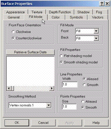 As
surfaces are represented by the set of polygonal objects they can be customized
using Fill Mode property pages. These property pages allow to define
front and back faces of the surfaces, the way front and back faces are drawn
(either as filled polygons, line stripes or simple points). Further
customization is achieved by a certain algorithm how the normals to the
surfaces are chosen.
As
surfaces are represented by the set of polygonal objects they can be customized
using Fill Mode property pages. These property pages allow to define
front and back faces of the surfaces, the way front and back faces are drawn
(either as filled polygons, line stripes or simple points). Further
customization is achieved by a certain algorithm how the normals to the
surfaces are chosen.
For complicated surface objects containing several sheets there is no unique way to define front and back faces. Since on the other hand this definition is important in connection to how surface reflects the light, we allow the swapping possibility between front and back of every surface sheet. The same is true for normal definitions. Usually only that part of surface with the normal pointing to the light source is highlighted. From the original data, the program computes the number of independent sheets that are present for given surface object. The corresponding tree control allows you to swap both front and back of every sheet and the normal direction. Special note has to be said about cross sections: since the number of independent sheets of the cross section depends on the contour value chosen (See 3D Curves & Surfaces: General Properties, the surface data should be extracted each time the cross-section value has been changed. The tree control also allows you to switch off certain surface sheets just by clearing the corresponding boxes at the tree controls. For complicated nested surfaces this is the only way to dress/undress the objects without doing any modifications of the original data.
The smoothness of the surface objects is another central issue. The smoothness of the surface is in general defined by the normal pointed perpendicular to the surface. It is further accounted for when computing the lighting properties of this object. The algorithm producing normals to the surface data points reflects the smoothness property. Three methods are implemented here: face normals will compute normals to every microface thus reflecting triangularized nature of the surfaces. Vertex normals 1 and 2 methods set the normals to every surface vertex rather than to microface which produces much more smoother objects in most cases.
You may convert every surface drawn into polygonal object. Use pop-up menu of the surface icon within the Object Explorer and use command Export As Object to make this conversion. This will create a polygonal object within the Polygons Database. Note that the way the normals are chosen to the surface will be stored and you will have no chance to use another normal generation algorithm after polygonal object is created and stored. If several sheets represent surface use the tree control to show/hide any of these sheets before storing the objects. Only surface sheets that are currently shown will be converted into polygonal object. See also the discussion Styles for Polygonal Objects.
D.8 Connecting Vertexes with 3D Curves
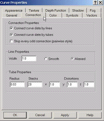 Use
Connection Property Page to specify connection line style between
vertexes of the 3D curve. You may choose to connect vertexes either by lines or
by tubes of a certain diameter. Also, a pairwise connection can be established
so that every pair (1-2,3-4, etc) of vertexes is connected. This can model
dashed line style for these objects.
Use
Connection Property Page to specify connection line style between
vertexes of the 3D curve. You may choose to connect vertexes either by lines or
by tubes of a certain diameter. Also, a pairwise connection can be established
so that every pair (1-2,3-4, etc) of vertexes is connected. This can model
dashed line style for these objects.
D.9 Coloring 3D Curves & Surfaces
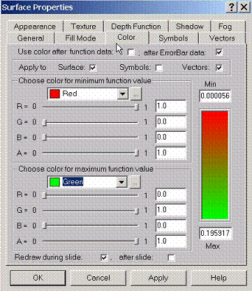
3D Curves/Surfaces and Cross-Sections can be colored not only by constant color controlled by the Appearance property page. Using Color property pages allows to associate the color index to every original data point. The color of every point can be either associated using the function values column or the error bar values column. The latter choice works for all 3D curves, surfaces and cross sections while the former one has no effect for cross-sections (since function value is constant on the surface). To use custom color for curves and surfaces, associate one color with the minimum function (error bar) value and another color to the maximum function (error bar value). The color index for given vertex which is associated with either function or error bar value will be computed using linear interpolation between the two edge color values. If the vertex function (error bar) value is outside the limit between maximum and minimum values, the corresponding edge values will be used. This method shows the possibility to visualize auxiliary functions additionally associated with the surface data points.
This coloring scheme can be
applied not only to the surface, but to the symbols drawn on top of the surface
and to the vectors drawn on top of the surface. To color symbols and/or vectors
according to this coloring scheme, make sure that symbol or vector own color is
set to its default value. See also Symbols property page and Vectors
property page
D.10 Using Symbols with 3D Curves &
Surfaces
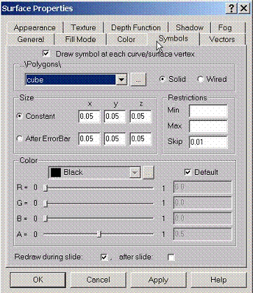 To
place symbol at every original data point use Symbols Property Page.
Different symbols can be chosen just from the polygonal objects database so
that virtually you may create and customize your own symbol style. Note however
that if the symbol objects are complicated, it may take a lot of computer time
to draw such objects at the surface data points.
To
place symbol at every original data point use Symbols Property Page.
Different symbols can be chosen just from the polygonal objects database so
that virtually you may create and customize your own symbol style. Note however
that if the symbol objects are complicated, it may take a lot of computer time
to draw such objects at the surface data points.
Once you have chosen the style for your symbols, you may need to rescale its size to properly adjust to the surface size. If the size of the surface is, for example, of the order 1, to draw symbols, which are the same objects of the original size of the order 1, you may need to rescale them by a factor of 100 to reach the desired effect. You can do such rescaling for x,y,z axes separately.
If error bar function data are associated with given surface you may choose to do such rescaling proportionally to this auxiliary function. In this way you have a possibility to visualize additional function associated with every data point.
If symbols appear too close to each other, the possibility to skip symbols which are lying closer that the certain distance is provided. This distance is set in the scene coordinates. if the scene itself is a cube with the coordinates from –1 to 1 along each direction, the skipping factor may vary from 0 to 2, and its default is 0.01.
Symbols can be colored by a
fixed color and also by the color set by the auxiliary function using the
errorbar association. To reach this effect, first select the default color for
the symbols. Then use Color property pageHIDD_SURFACE_PROPERTIES_COLOR to set up the coloring scheme and select
“Apply to Symbols”.
D.11 Using Vectors with 3D Curves &
Surfaces
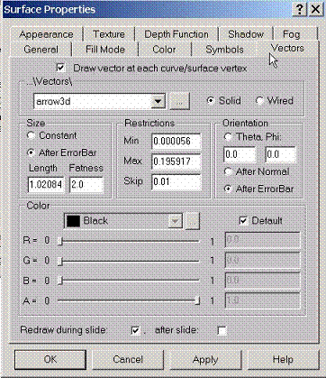 To
place vector at every original data point use Vectors Property Page.
Different vectors can be chosen just from the polygonal objects database
appeared in the …/Vectors/ folder so that virtually you may create and
customize your own vector style. Note however that if the vector objects are
complicated, it may take a lot of computer time to draw such objects at the
surface data points.
To
place vector at every original data point use Vectors Property Page.
Different vectors can be chosen just from the polygonal objects database
appeared in the …/Vectors/ folder so that virtually you may create and
customize your own vector style. Note however that if the vector objects are
complicated, it may take a lot of computer time to draw such objects at the
surface data points.
The orientation of the vector is initially assumed to be along vertical axis pointing to the top. If the coordinate system associated with the scene is horizontal right (x), vertical top (y), and screen near (z), this orientation is along scene y axis.
Once you have chosen the style for your vectors, you will need to rescale its length, fatness, and orientation to properly display vector field associated with the surface. Several situations are possible depending on whether errorbar function is associated with the surface.
(i)
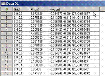 If
no errorbar function is available, the vectors can be drawn at certain length
and under certain orientation set either by the angles theta and phi, or as
normals to the surface (the latter option is disabled for 3D curves)
If
no errorbar function is available, the vectors can be drawn at certain length
and under certain orientation set either by the angles theta and phi, or as
normals to the surface (the latter option is disabled for 3D curves)
(ii) If errorbar function is available for every point of the surface, the length of each vector can be set proportional to the errorbar. Again, rescaling the length of the vector maybe a useful option since min and max values of the errorbar function can be arbitrary.
(iii) If errorbar function is set as a vector field, i.e. 3 components are available, not only the length but also orientation of the vector can be set according the errorbar function.
If vectors appear too close to each other, the possibility to skip vectors which are lying closer that the certain distance is provided. This distance is set in the scene coordinates. if the scene itself is a cube with the coordinates from –1 to 1 along each direction, the skipping factor may vary from 0 to 2, and its default is 0.01
Vectors can be colored by a fixed color and also by the color set by the auxiliary function using the errorbar association. To reach this effect, first select the default color for the vectors. Then use Color property pageHIDD_SURFACE_PROPERTIES_COLOR to set up the coloring scheme and select “Apply to Vectors”.
E.1 Light Properties: Spot
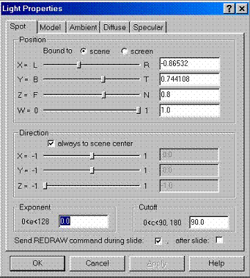 In
RGBA mode, the lighted color of a vertex is the sum of the material emission
intensity, the product of the material ambient reflectance and the lighting
model full-scene ambient intensity, and the contribution of each enabled light
source. Each light source contributes the sum of three terms: ambient, diffuse,
and specular. The ambient light source contribution is the product of the
material ambient reflectance and the light's ambient intensity. The diffuse
light source contribution is the product of the material diffuse reflectance,
the light's diffuse intensity, and the dot product of the vertex's normal with
the normalized vector from the vertex to the light source. The specular light
source contribution is the product of the material specular reflectance, the
light's specular intensity, and the dot product of the normalized vertex-to-eye
and vertex-to-light vectors, raised to the power of the shininess of the
material. All three light source contributions are attenuated equally based on
the distance from the vertex to the light source and on light source direction,
spread exponent, and spread cutoff angle. All dot products are replaced with
zero if they evaluate to a negative value.
In
RGBA mode, the lighted color of a vertex is the sum of the material emission
intensity, the product of the material ambient reflectance and the lighting
model full-scene ambient intensity, and the contribution of each enabled light
source. Each light source contributes the sum of three terms: ambient, diffuse,
and specular. The ambient light source contribution is the product of the
material ambient reflectance and the light's ambient intensity. The diffuse
light source contribution is the product of the material diffuse reflectance,
the light's diffuse intensity, and the dot product of the vertex's normal with
the normalized vector from the vertex to the light source. The specular light
source contribution is the product of the material specular reflectance, the
light's specular intensity, and the dot product of the normalized vertex-to-eye
and vertex-to-light vectors, raised to the power of the shininess of the
material. All three light source contributions are attenuated equally based on
the distance from the vertex to the light source and on light source direction,
spread exponent, and spread cutoff angle. All dot products are replaced with
zero if they evaluate to a negative value.
Position of light spot
is given by three values in the coordinate system of the scene and is
controlled by the Spot property page. On top of it, there is a w component
of the position: if it is 0.0, the light is treated as a directional source. In
general, the position of the light is transformed by the 4*4 modelview matrix
and is stored in eye coordinates. Diffuse and specular lighting calculations
take the lights direction, but not its actual position, into account, and
attenuation is disabled. Otherwise, diffuse and specular lighting calculations
are based on the actual location of the light in eye coordinates, and
attenuation is enabled.
By default, the program places the
light source in the near plane of the Scene and directs it to the center. Light
direction is controlled by the vector in the scene coordinate system. It is
significant only when the spot cutoff is not equal to 180. The latter is the cutoff
parameter which is a single integer or floating-point value that specifies the
maximum spread angle of a light source. Integer and floating-point values are
mapped directly. Only values in the range [0,90], and the special value 180,
are accepted. If the angle between the direction of the light and the direction
from the light to the vertex being lighted is greater than the spot cutoff
angle, then the light is completely masked. Otherwise, its intensity is
controlled by the spot exponent and the attenuation factors. The spot cutoff
equal to 180 results in uniform light distribution.
There exist three light attenuation
factors which are controlled by integer or floating-point values. Only
nonnegative values are accepted. If the light is positional, rather than
directional, its intensity is attenuated by the reciprocal of the sum of: the
constant factor, the linear factor multiplied by the distance between the light
and the vertex being lighted, and the quadratic factor multiplied by the square
of the same distance. The default attenuation factors are (1,0,0), resulting in
no attenuation.
E.2 Light Properties: Model
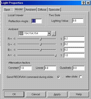 In RGBA mode, the
lighted color of a vertex is the sum of the material emission intensity, the
product of the material ambient reflectance and the lighting model full-scene
ambient intensity, and the contribution of each enabled light source. Each
light source contributes the sum of three terms: ambient, diffuse, and
specular. The ambient light source contribution is the product of the material
ambient reflectance and the light's ambient intensity. The diffuse light source
contribution is the product of the material diffuse reflectance, the light's
diffuse intensity, and the dot product of the vertex's normal with the
normalized vector from the vertex to the light source. The specular light
source contribution is the product of the material specular reflectance, the
light's specular intensity, and the dot product of the normalized vertex-to-eye
and vertex-to-light vectors, raised to the power of the shininess of the
material. All three light source contributions are attenuated equally based on the
distance from the vertex to the light source and on light source direction,
spread exponent, and spread cutoff angle. All dot products are replaced with
zero if they evaluate to a negative value.
In RGBA mode, the
lighted color of a vertex is the sum of the material emission intensity, the
product of the material ambient reflectance and the lighting model full-scene
ambient intensity, and the contribution of each enabled light source. Each
light source contributes the sum of three terms: ambient, diffuse, and
specular. The ambient light source contribution is the product of the material
ambient reflectance and the light's ambient intensity. The diffuse light source
contribution is the product of the material diffuse reflectance, the light's
diffuse intensity, and the dot product of the vertex's normal with the
normalized vector from the vertex to the light source. The specular light
source contribution is the product of the material specular reflectance, the
light's specular intensity, and the dot product of the normalized vertex-to-eye
and vertex-to-light vectors, raised to the power of the shininess of the
material. All three light source contributions are attenuated equally based on the
distance from the vertex to the light source and on light source direction,
spread exponent, and spread cutoff angle. All dot products are replaced with
zero if they evaluate to a negative value.
The following light models are used which are controlled by
the Model property page: LOCAL VIEWER MODEL is controlled by the
parameter which is a single integer or floating-point value that specifies how
specular reflection angles are computed. If params is 0, specular
reflection angles take the view direction to be parallel to and in the
direction of the –z axis, regardless of the location of the vertex in eye
coordinates. Otherwise specular reflections are computed from the origin of the
eye coordinate system. The default is 0. TWO SIDE MODEL is controlled by the
parameter which is a single integer or floating-point value that specifies
whether one- or two-sided lighting calculations are done for polygons. It has
no effect on the lighting calculations for points, lines, or bitmaps. If params
is 0 (or 0.0), one-sided lighting is specified, and only the front
material parameters are used in the lighting equation. Otherwise, two-sided
lighting is specified. In this case, vertices of back-facing polygons are
lighted using the back material parameters, and have their normals
reversed before the lighting equation is evaluated. Vertices of front-facing
polygons are always lighted using the front material parameters, with no
change to their normals. The default is 0. AMBIENT MODEL is controlled by the
four integer or floating-point values that specify the ambient RGBA intensity
of the entire scene. Integer values are mapped linearly such that the most
positive representable value maps to 1.0, and the most negative representable
value maps to –1.0. Floating-point values are mapped directly. Neither integer
nor floating-point values are clamped. The default ambient scene intensity is
(0.2, 0.2, 0.2, 1.0).
E.3 Light Properties: Ambient Component
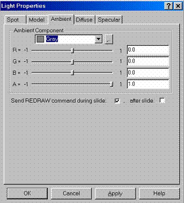 In
RGBA mode, the lighted color of a vertex is the sum of the material emission
intensity, the product of the material ambient reflectance and the lighting
model full-scene ambient intensity, and the contribution of each enabled light
source. Each light source contributes the sum of three terms: ambient, diffuse,
and specular. The ambient light source contribution is the product of the
material ambient reflectance and the light's ambient intensity. The diffuse
light source contribution is the product of the material diffuse reflectance,
the light's diffuse intensity, and the dot product of the vertex's normal with
the normalized vector from the vertex to the light source. The specular light
source contribution is the product of the material specular reflectance, the
light's specular intensity, and the dot product of the normalized vertex-to-eye
and vertex-to-light vectors, raised to the power of the shininess of the
material. All three light source contributions are attenuated equally based on
the distance from the vertex to the light source and on light source direction,
spread exponent, and spread cutoff angle. All dot products are replaced with
zero if they evaluate to a negative value.
In
RGBA mode, the lighted color of a vertex is the sum of the material emission
intensity, the product of the material ambient reflectance and the lighting
model full-scene ambient intensity, and the contribution of each enabled light
source. Each light source contributes the sum of three terms: ambient, diffuse,
and specular. The ambient light source contribution is the product of the
material ambient reflectance and the light's ambient intensity. The diffuse
light source contribution is the product of the material diffuse reflectance,
the light's diffuse intensity, and the dot product of the vertex's normal with
the normalized vector from the vertex to the light source. The specular light
source contribution is the product of the material specular reflectance, the
light's specular intensity, and the dot product of the normalized vertex-to-eye
and vertex-to-light vectors, raised to the power of the shininess of the
material. All three light source contributions are attenuated equally based on
the distance from the vertex to the light source and on light source direction,
spread exponent, and spread cutoff angle. All dot products are replaced with
zero if they evaluate to a negative value.
Ambient RGBA intensity of the light is controlled by Ambient property page. The default ambient light intensity is (0.0, 0.0, 0.0, 1.0). Integer RGB values from 0 to 255 are mapped linearly to the real values such that the most positive representable value maps to 1.0, and the most negative representable value maps to –1.0.
E.4 Light Properties: Diffuse Component
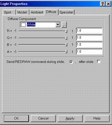 In
RGBA mode, the lighted color of a vertex is the sum of the material emission
intensity, the product of the material ambient reflectance and the lighting
model full-scene ambient intensity, and the contribution of each enabled light
source. Each light source contributes the sum of three terms: ambient, diffuse,
and specular. The ambient light source contribution is the product of the
material ambient reflectance and the light's ambient intensity. The diffuse
light source contribution is the product of the material diffuse reflectance, the
light's diffuse intensity, and the dot product of the vertex's normal with the
normalized vector from the vertex to the light source. The specular light
source contribution is the product of the material specular reflectance, the
light's specular intensity, and the dot product of the normalized vertex-to-eye
and vertex-to-light vectors, raised to the power of the shininess of the
material. All three light source contributions are attenuated equally based on
the distance from the vertex to the light source and on light source direction,
spread exponent, and spread cutoff angle. All dot products are replaced with
zero if they evaluate to a negative value.
In
RGBA mode, the lighted color of a vertex is the sum of the material emission
intensity, the product of the material ambient reflectance and the lighting
model full-scene ambient intensity, and the contribution of each enabled light
source. Each light source contributes the sum of three terms: ambient, diffuse,
and specular. The ambient light source contribution is the product of the
material ambient reflectance and the light's ambient intensity. The diffuse
light source contribution is the product of the material diffuse reflectance, the
light's diffuse intensity, and the dot product of the vertex's normal with the
normalized vector from the vertex to the light source. The specular light
source contribution is the product of the material specular reflectance, the
light's specular intensity, and the dot product of the normalized vertex-to-eye
and vertex-to-light vectors, raised to the power of the shininess of the
material. All three light source contributions are attenuated equally based on
the distance from the vertex to the light source and on light source direction,
spread exponent, and spread cutoff angle. All dot products are replaced with
zero if they evaluate to a negative value.
Diffuse RGBA intensity of the light is controlled by Diffuse property page. The default diffuse light intensity is (0.0, 0.0, 0.0, 1.0). Integer RGB values from 0 to 255 are mapped linearly to the real values such that the most positive representable value maps to 1.0, and the most negative representable value maps to –1.0.
E.5 Light Properties: Specular Component
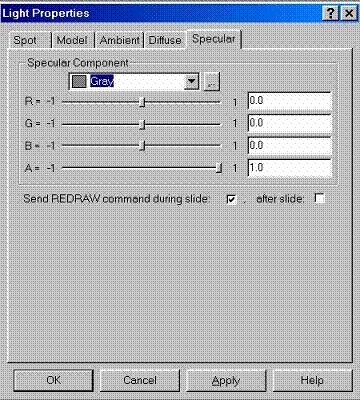 In
RGBA mode, the lighted color of a vertex is the sum of the material emission
intensity, the product of the material ambient reflectance and the lighting
model full-scene ambient intensity, and the contribution of each enabled light
source. Each light source contributes the sum of three terms: ambient, diffuse,
and specular. The ambient light source contribution is the product of the
material ambient reflectance and the light's ambient intensity. The diffuse
light source contribution is the product of the material diffuse reflectance,
the light's diffuse intensity, and the dot product of the vertex's normal with
the normalized vector from the vertex to the light source. The specular light
source contribution is the product of the material specular reflectance, the
light's specular intensity, and the dot product of the normalized vertex-to-eye
and vertex-to-light vectors, raised to the power of the shininess of the
material. All three light source contributions are attenuated equally based on
the distance from the vertex to the light source and on light source direction,
spread exponent, and spread cutoff angle. All dot products are replaced with
zero if they evaluate to a negative value.
In
RGBA mode, the lighted color of a vertex is the sum of the material emission
intensity, the product of the material ambient reflectance and the lighting
model full-scene ambient intensity, and the contribution of each enabled light
source. Each light source contributes the sum of three terms: ambient, diffuse,
and specular. The ambient light source contribution is the product of the
material ambient reflectance and the light's ambient intensity. The diffuse
light source contribution is the product of the material diffuse reflectance,
the light's diffuse intensity, and the dot product of the vertex's normal with
the normalized vector from the vertex to the light source. The specular light
source contribution is the product of the material specular reflectance, the
light's specular intensity, and the dot product of the normalized vertex-to-eye
and vertex-to-light vectors, raised to the power of the shininess of the
material. All three light source contributions are attenuated equally based on
the distance from the vertex to the light source and on light source direction,
spread exponent, and spread cutoff angle. All dot products are replaced with
zero if they evaluate to a negative value.
Specular RGBA intensity of the light is controlled by Specular property page. The default specular light intensity is (0.0, 0.0, 0.0, 1.0). Integer RGB values from 0 to 255 are mapped linearly to the real values such that the most positive representable value maps to 1.0, and the most negative representable value maps to –1.0.
F.1 Customizing Data Tables: General Properties
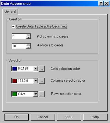 Use
General Property Page, to customize table appearance, initial #’s for
columns and rows, selections colors, etc
Use
General Property Page, to customize table appearance, initial #’s for
columns and rows, selections colors, etc
F.2 Customizing Plot Pages: General Properties
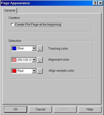 Use
General Property Page, to customize plots pages appearance &
behavior, selections colors, etc
Use
General Property Page, to customize plots pages appearance &
behavior, selections colors, etc
F.3 Customizing Scenes: General Properties
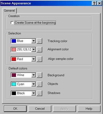 Use
General Property Page, to customize scenes appearance & behavior,
selections colors, etc
Use
General Property Page, to customize scenes appearance & behavior,
selections colors, etc
F.4 Customizing Scenes: OpenGL Properties
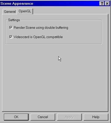 Use
OpenGL Property Page, to select whether your video card supports OpenGL
instructions and whether rendering should be done using double buffering mode.
When double buffering is used the image is first drawn onto the back buffer and
then shown on the front buffer (screen). This avoids screen flicking during
redrawing operations.
Use
OpenGL Property Page, to select whether your video card supports OpenGL
instructions and whether rendering should be done using double buffering mode.
When double buffering is used the image is first drawn onto the back buffer and
then shown on the front buffer (screen). This avoids screen flicking during
redrawing operations.